[Torrey, Ian, Daniel, Sander, Lee]
Introduction
We have been struggling for a while to figure out a configuration for a stable cavity lock using only the piezo mirrors. In an effort to troubleshoot, we want to take a transfer function of just the piezo (hp). We can't do this directly while the cavity is aligned and locked so we have to be a little clever about it. Below is a how we go about doing this.
Set up and methods
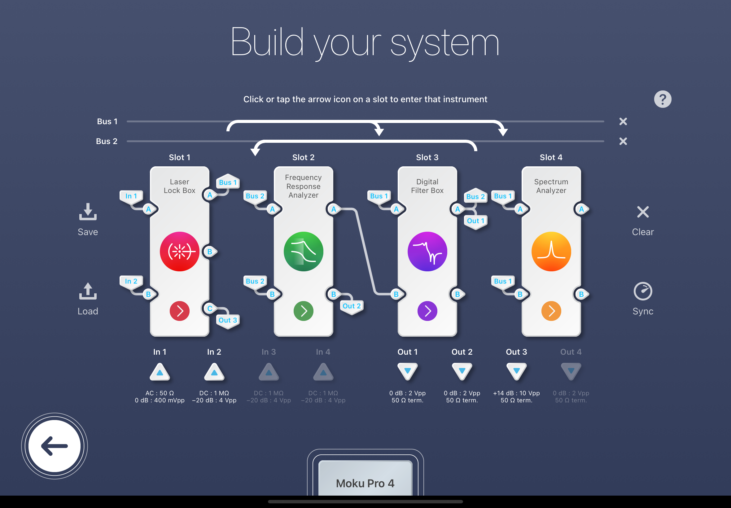
In the moku multi-instrument mode we can set up a combination of transfer functions to achieve the piezo transfer function. As seen in this, we lock the cavity with the laser. The digital filter box is used as a summer. Output 1 is used to control the DC modulation port of the ULN15TK laser and Output 2 is used for the cavity piezo. Output 3 is the 50 MHz signal used for demod. Input 1 is the newport 1811 high bandwidth PD in reflection of the cavity. Input 2 is the GE lower bandwidth PD in transmission of the cavity. Two transfer functions are set up in this configuration:
- Fast controller (laser frequency controller) divided by excitation to laser frequency.
- Fast controller (laser frequency controller) divided by excitation to the laser piezo.
We can reduce this diagram to a clearer picture of the control systems in play using a Signal Flow Graph (alternate picture to the more common block diagrams). This reduction can be seen as signal_flow.pdf. From this diagram we can see the open loop gain G can be written as \[G = H_1*F*H_2*\alpha.\] We can subsequently reduce our individual transfer functions into smaller diagrams, seen in reduction_A.pdf and reduction_B.pdf. From these it is a little easier to write down the equations for our transfer functions in terms of G and individual components. From reduction_A.pdf we see that,
\[T_p = V_{LF} \] and \[V_{VL} = A + G V_{LF}.\] This means \[\frac{T_p}{A} = \frac{1}{1-G}.\] For now we will call this measurement one, or \[M_1 = \frac{T_p}{A} = \frac{1}{1-G}.\] Similarly from reduction_B.pdf,
\[T_p = \frac{H_p}{H_2} \frac{G}{1-G} B.\] Again lets call this measurement two, so \[M_2 = \frac{T_p}{B} = \frac{H_p}{H_2} \frac{G}{1-G}.\]
Take the ratio of M2 and M1:
\[\frac{M_2}{M_1} = G \frac{H_P}{H_2}\]. Substitute the above expression for G and solve for H2,
\[H_p = \frac{M_2}{M_1} * \frac{1}{H_1 F \alpha}\].
This is a nice form as every variable can be obtained experimentally or is known already.
- M1 and M2 are our measured transfered functions.
- F is the filter used in the digital filter box which at the time of measurement 0 db for all frequencies so trivially F=1.
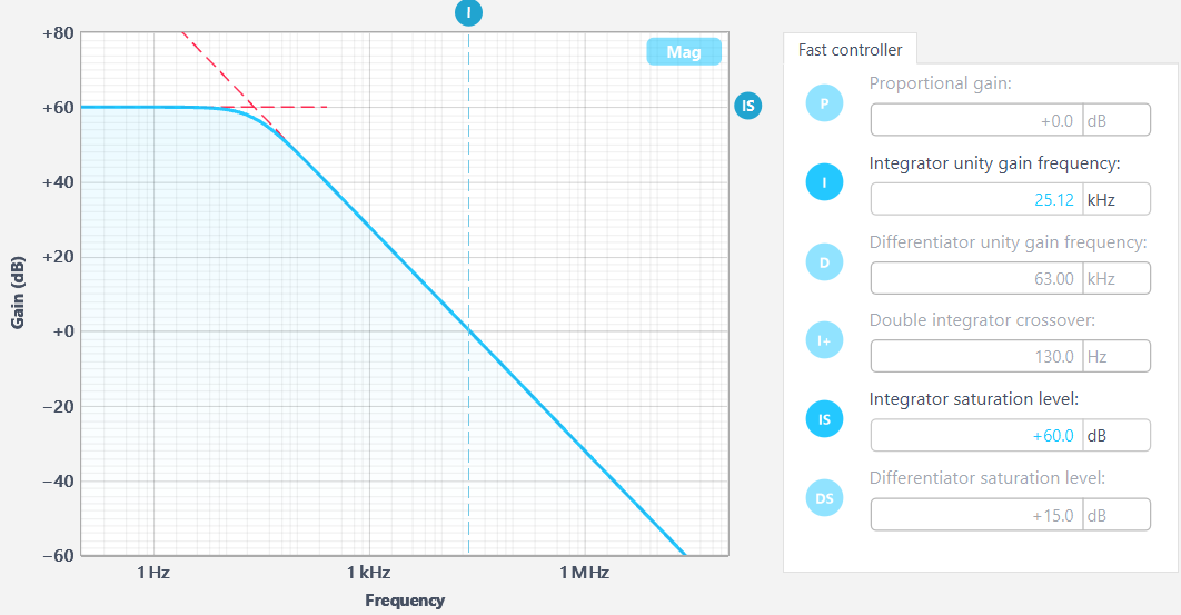
- H_1 is the shape of the fast controller of the laser lock box. This is slightly annoying to recreate as there is no way to download the shape of the loop directly from the fast controller of the laser lock box. I get around this by recreating it in python using scipy. Most scipy functions seem to want the order of the filter and cutoff frequency; cutoff frequency being a problem as the controller shape is defined by the UGF and not cutoff frequency (ex: fast_controller_example.png). A conversion can be made but slightly annoying. Jeff is currently very close to being done with a script that will take these 6 inputs and recreate the shape of the controller in python.
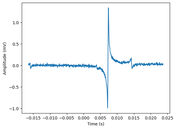
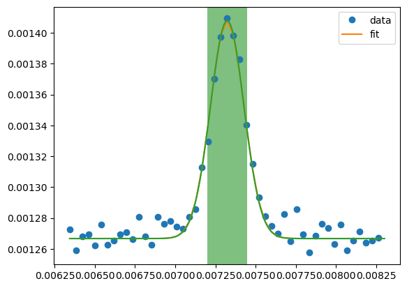
- Alpha is the conversion from Hz into Volts from the laser frequency to the PDH lock. This is found by the ratio of the amplitude of the error signal in the PDH lock and the cavity bandwidth. The error_signal amplitude can be found trivially by putting one of the moku test points at the error signal. The cavity bandwidth can be derived or measured in a few different ways. The method we went with was to scan the laser frequency to see 0,0 peaks in the TRANS PD. This peak will have some width, from which the FWHM in time (delta t). In order to convert this to a frequency we do the following conversion:
\[\mathrm{BW(Hz)} = \Delta t * \frac{2 A}{T} * \frac{2 mA}{V} \frac{5 pm}{20 mA} \frac{c}{\lambda^2}\]
- 2A/T converts the width of the peak from time to volts.
- 2 mA}/V is the conversion of the DC modulation quoted on the thorlabs website from input voltage to pump current modulation.
- 5 pm/20 mA is how much the laser wavelength changes given some amount of change in pump current. Note that this is only true in the linear regime and is not true everywhere. For small changes, as is the case here, it is true.
- c/\lambda^2is the derivative df/d lambda of f=c/lambda to convert from meters to frequency.
From the data collected this yields approximately 307 kHz bandwidth for the cavity with the low reflectivity mirrors (R ~~ 99%).
Results
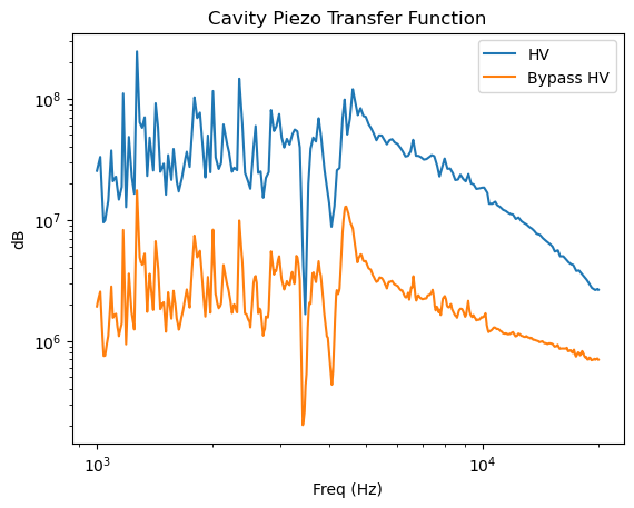
The final result of \[H_p = \frac{M_2}{M_1} * \frac{1}{H_1 F \alpha}\] yields result.png. I think there is a scaling factor off somewhere but the shape makes sense. Also something to look into is the low quality of the data at low frequencies, of which Lee has given me ideas on how to correct this. We cannot simply drive these things harder.

[Ian, Torrey]
Update to the above.
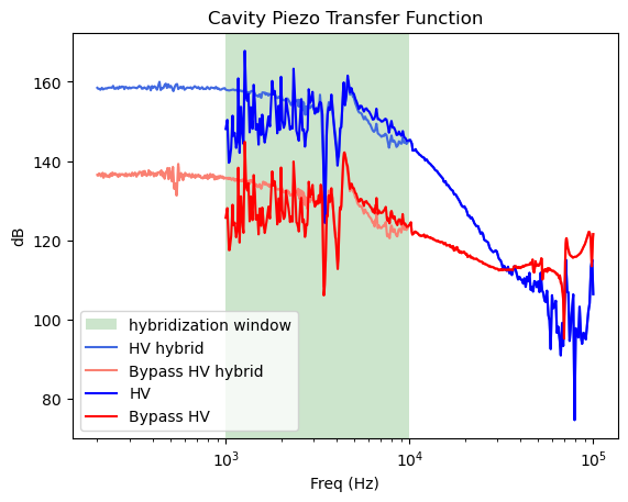
As seen from the final result above, the low frequency data is garbage. Eventually we will want to be able to shape a loop at all frequencies. To get around this we have approximated the low frequencies as just the shape of the fast controller. We then wrote some code to stitch them together in a given frequency range, where below this range M1 is given as just the fast controller, in this window it is given as a combination of the two, and above it it is given as just the measured data. This window is represented by the shaded green in result_updated.png. I will post this script to the log in a follow up post once I have cleaned it up.
We should be able to quickly model the cavity piezo transfer function at all frequencies based on a few inputs now.
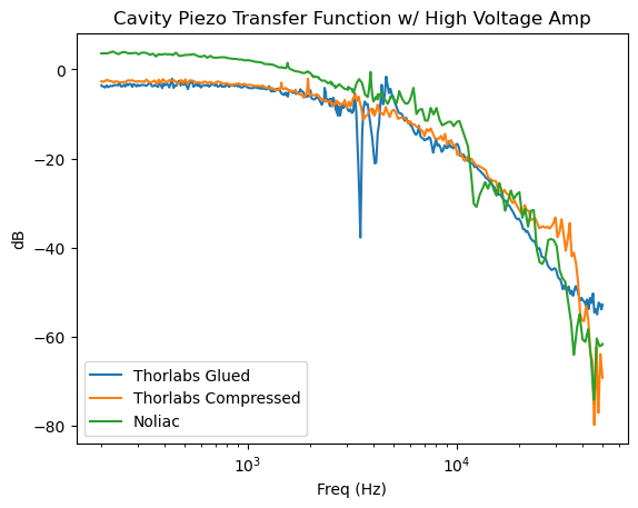
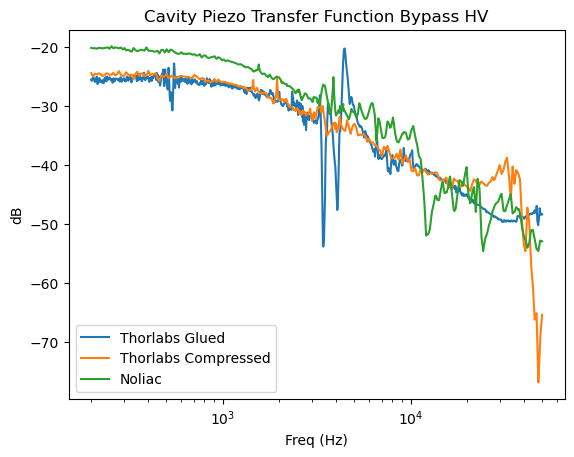
[Ian, Alex, Torrey]
The previous data taken was with the thorlabs piezo that is glued to the mirror. We swapped out M3 with the noliac piezo and thorlabs piezo in the compressed configuration, realigned both times, and took the same data and ran it through my code. The result of which can be seen in the above plots. I plan on doing these same measurements with a square noliac piezo and the small thorlabs piezo in compressed configuration.