I've written a notebook which takes second order section coefficents, sets the digital filter box, measures the frequency response, and compares it to a pythoncontrol model. The notebook is labeled "DigitalFilterBox_TransferFunction" and is saved in the MOKU_scripts folder.
The filter measured is given as an example in the API documentation, and described as "an 8th order Direct-form 1 Chebyshev type 2 IIR filter with a normalized stopband frequencyof 0.2 pi rad/sample and a stopband attenuation of 40 dB." The magnitude of the model and measured tranfer functions looks the same to eye, but the phases do not match. I expect that internal delays in the Moku will cause phase loss, but I'm not sure how big to expect this effect to be. Additionally the phase curves move in different directions, and I am not sure how to explain that discrepancy.
Script outline:
Define the IIR filter as a series of second-order sections. The Moku wants these coefficents in a form described in the user manual (unfortunately it is not documented in the API documentation). Each IIR filter can have a maximum of 4 second order sections. You also have to give the Moku a sampling frequency which is one of the 3 allowed frequencies: 39.06MHz, 4.883MHz, 305.2kHz for the Moku Pro.
Measure the IIR filter with the frequency response analyzer. Define a frequency sweep and execute it, making sure to wait until the sweep is complete to pull the data.
Define the pythoncontrol model of the filter. Python control allows for discrete time transfer functions by passing it a sampling time. (s -> z^-1) The total transfer function is calculated as the second order sections in series.
Most of the data manipulations are done with dataframes, and the plotting with Vega Altair. Another example of using Altair to plot multiple transfer functions is in the notebook "plotting_sos"
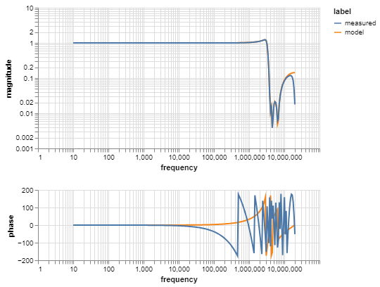


Very cool. Do you have a screenshot or a diagram of how you're taking these TFs? Curious about the phase difference.
Here's the multi instrument setup.