[Ian, Torrey, Jeff, Daniel]
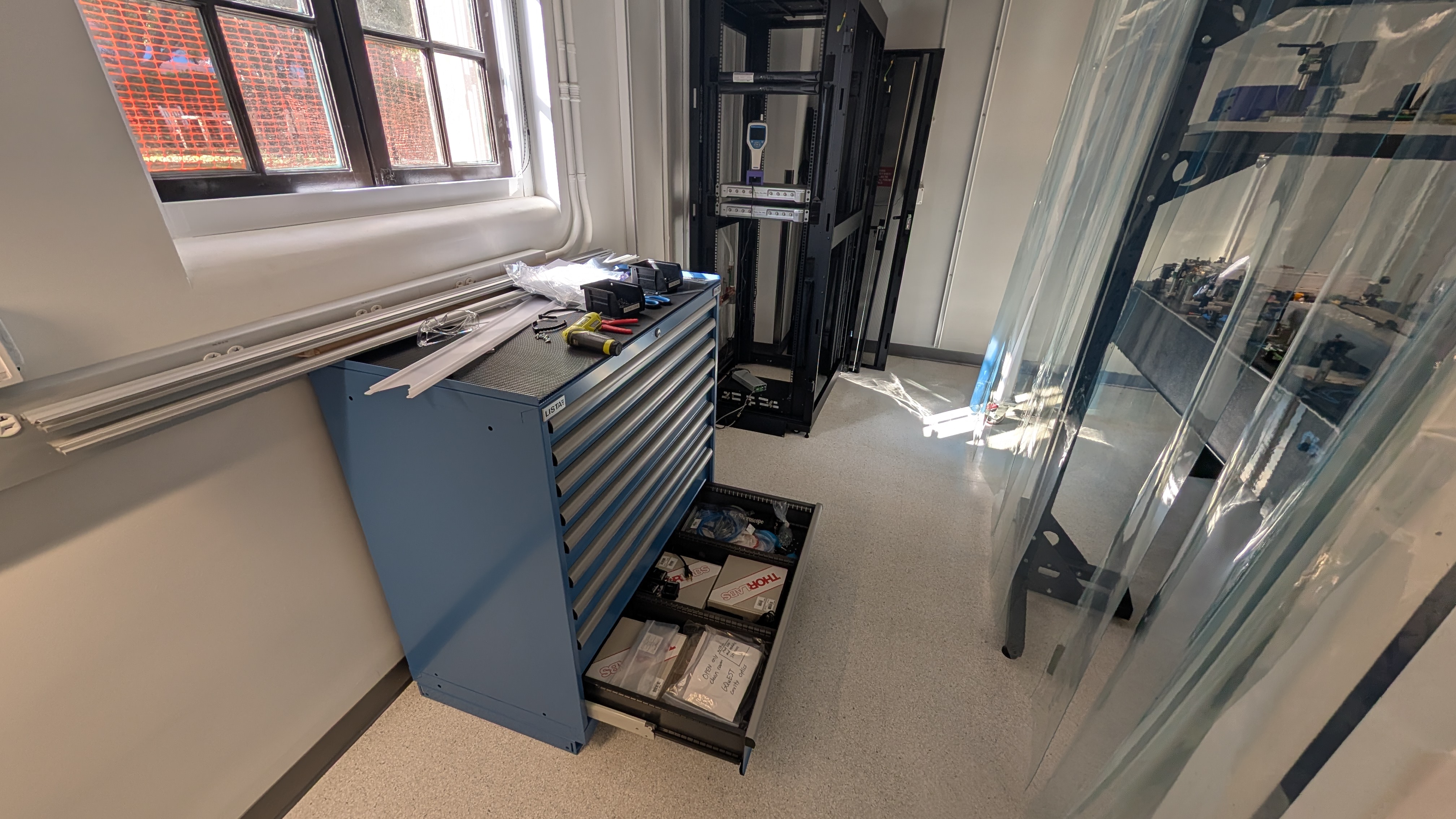
Since we are limited by the 1 meter length of the fiber coming out of the amplifier, we decided to move the Laser and amplifier below the table from its current position on the shelves above the optical table. The thought is that that space will be very valuable and since we don't plan on touching the laser much we would rather put it under the table. Jeff found a rack that will fit under the table and we plan to put it under the South side of the table. This will give enough room to let the short fiber get to the top of the table. The amplifier will be mounted on the top of the short rack and the seed laser and polarizing paddles will be below it on a ThorLabs rack mount bread board. Daniel is mocking up how all the components will fit into the box.
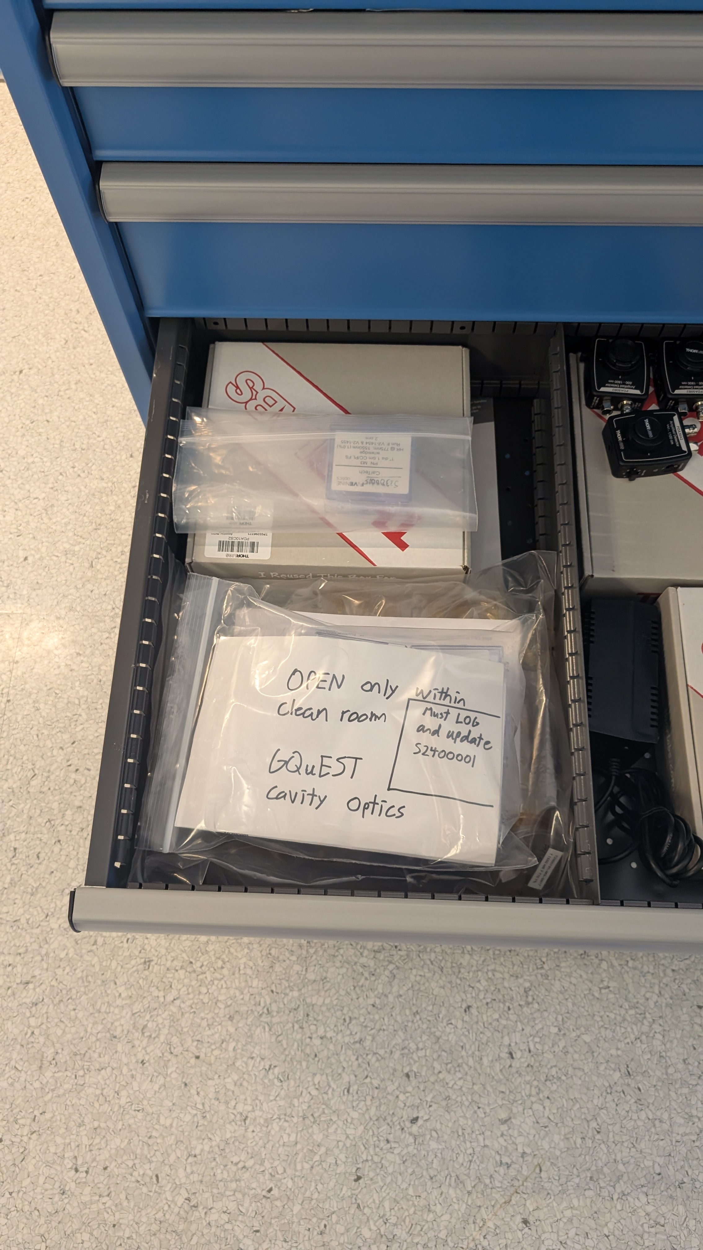
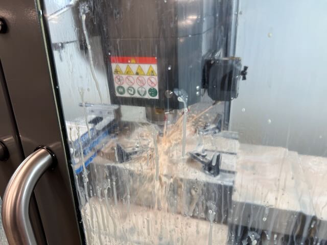
We also want to mock up a way to protect the fiber coming out of the amplifier. I want to put a plate in front of the rack mountable amplifier that attaches to the rack. This full face plate will protect any of the cables from getting kicked.
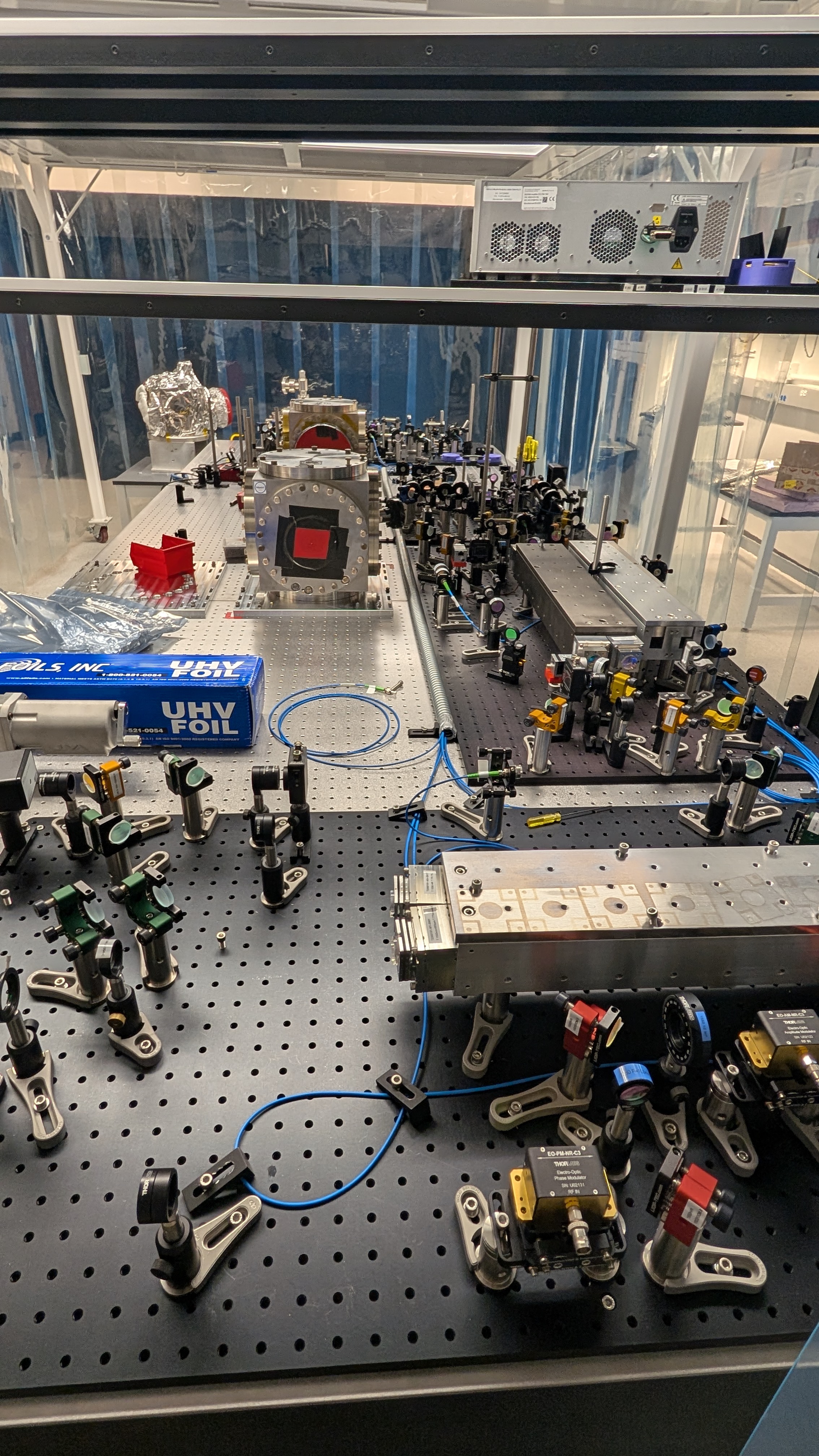
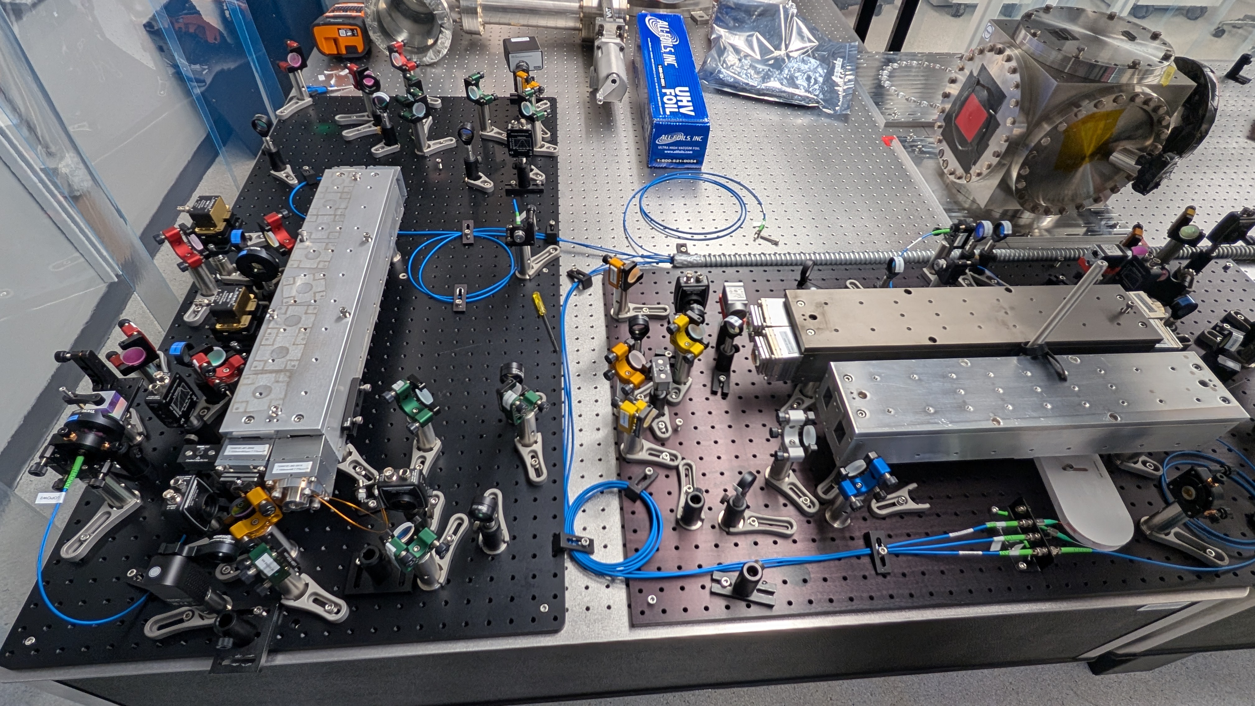
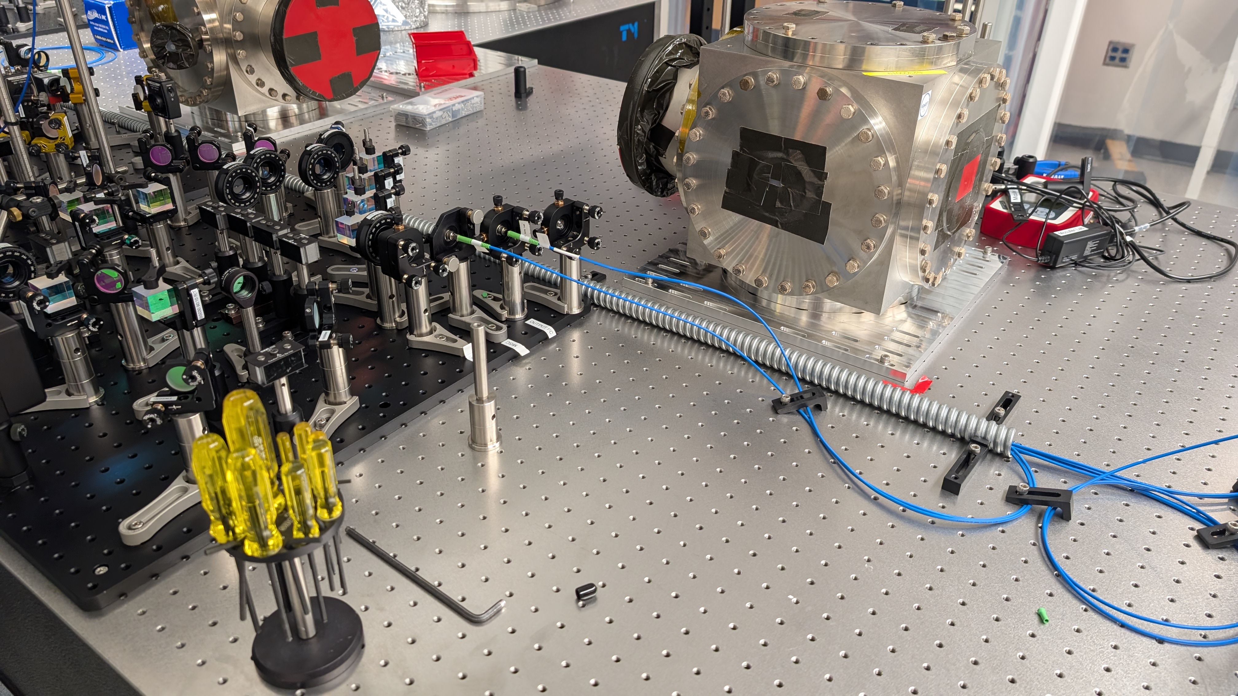
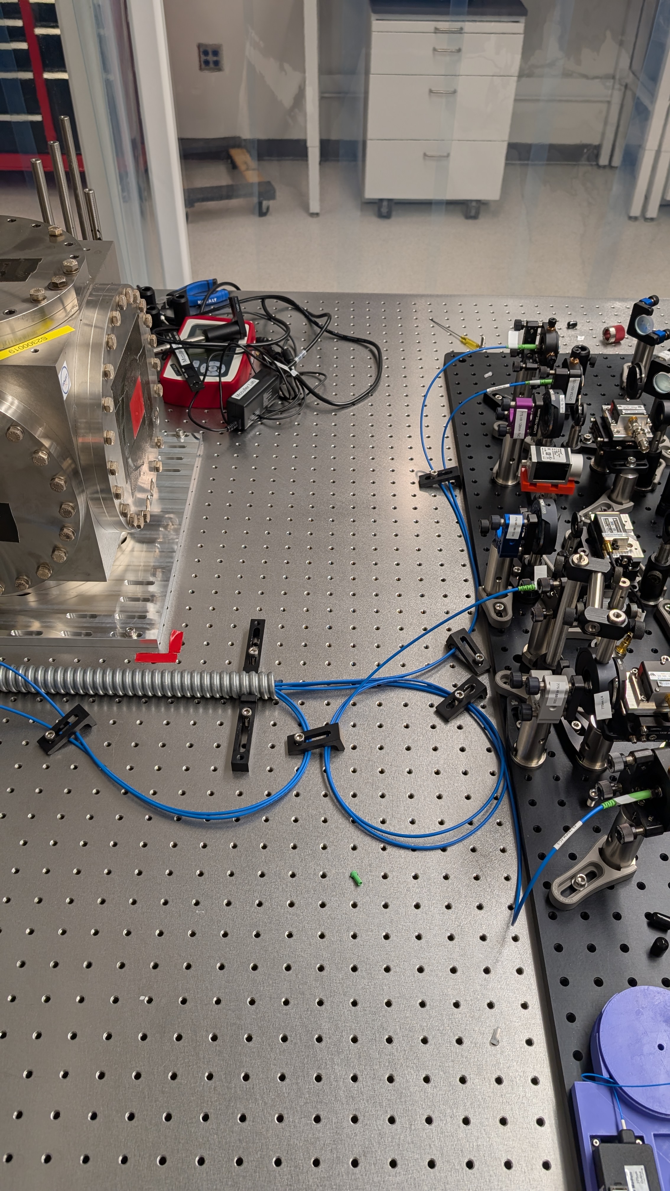


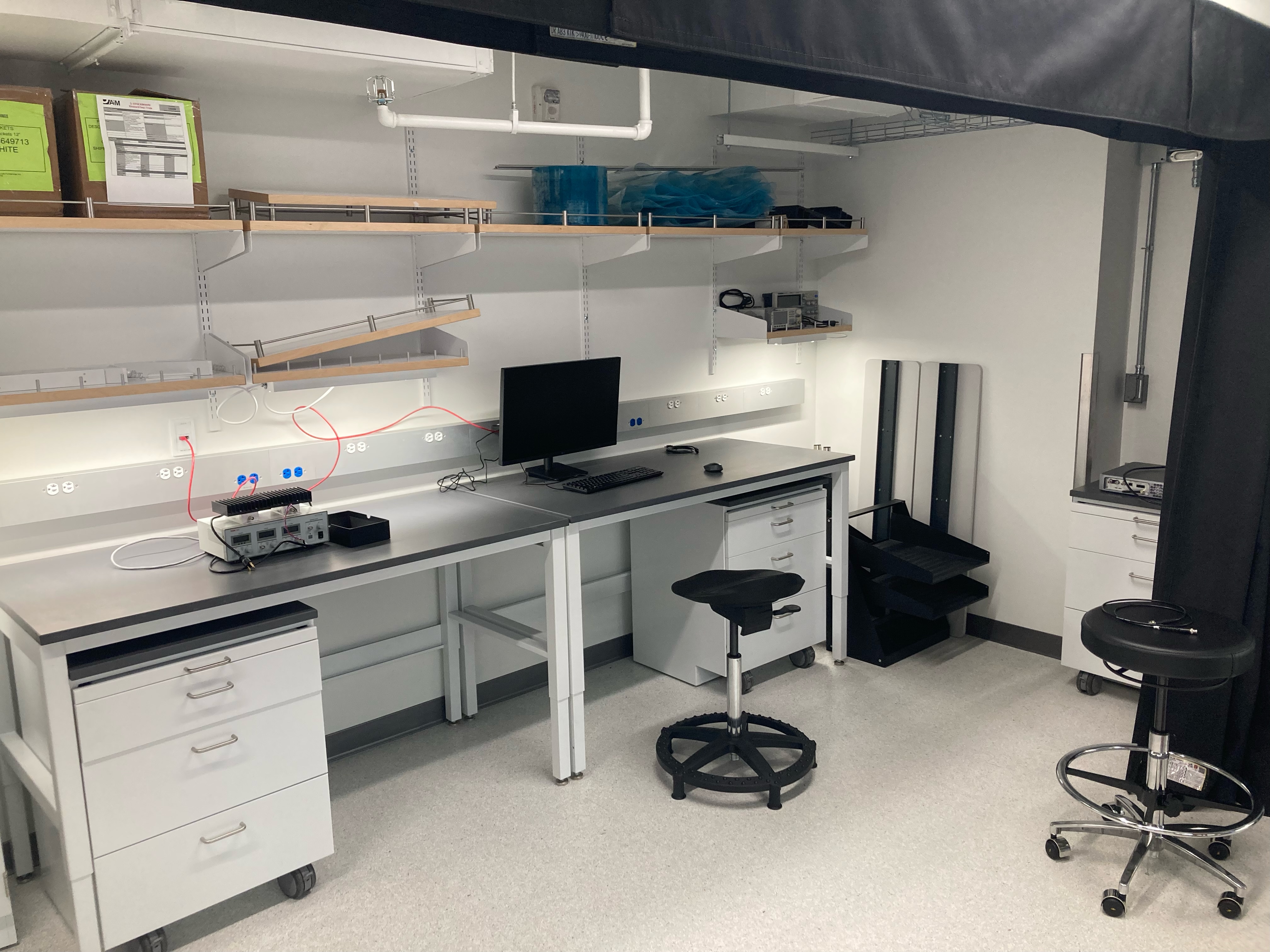
See this attached setup. This is the same laser schematic as is currently in place, but the components are moved around to save space.