Jeffrey Wack - posted 18:09, Tuesday 02 April 2024 - last comment - 18:10, Tuesday 02 April 2024(11519)
RFSoC 4x2 delay
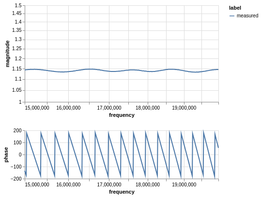
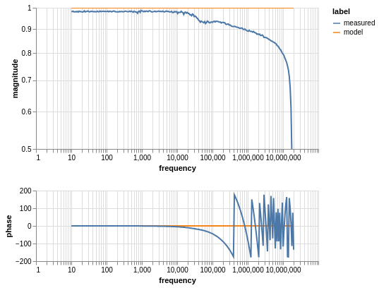
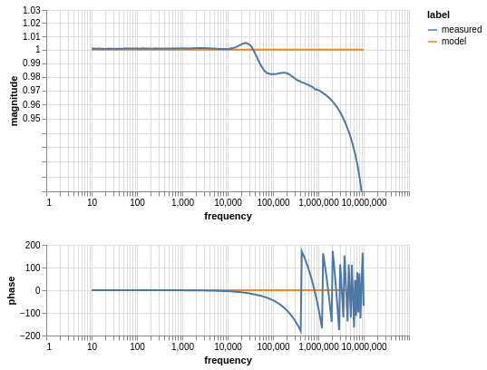
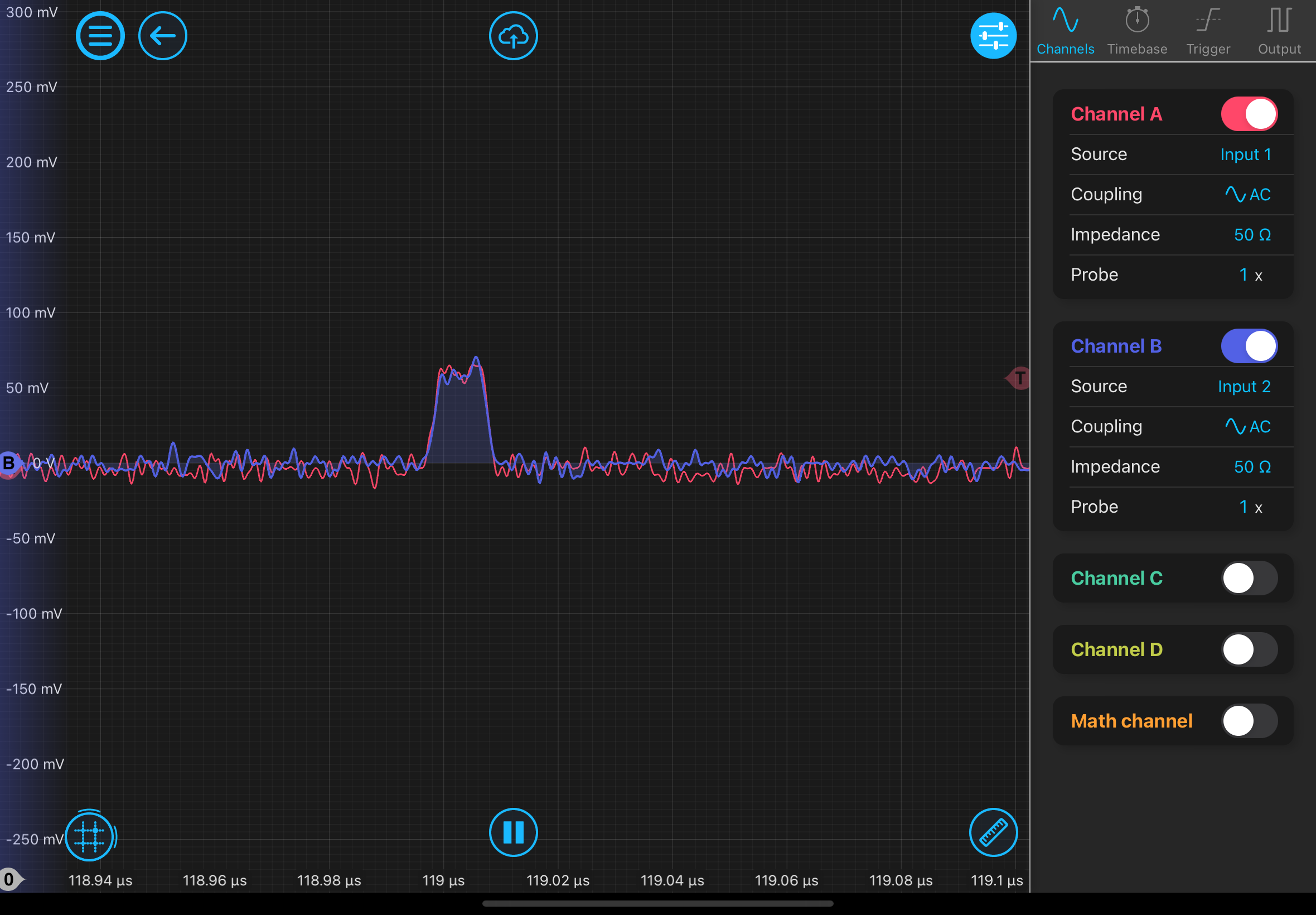
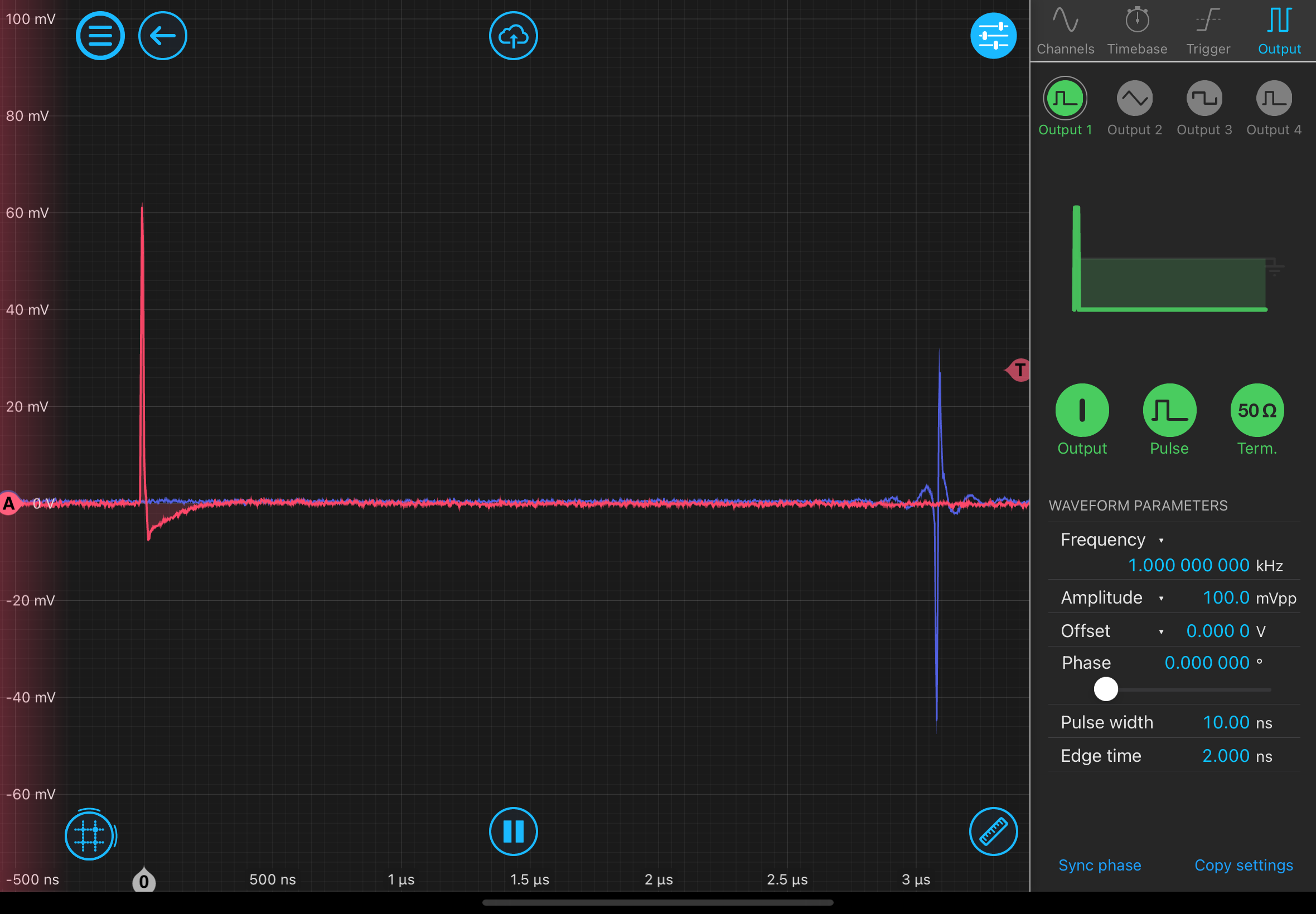
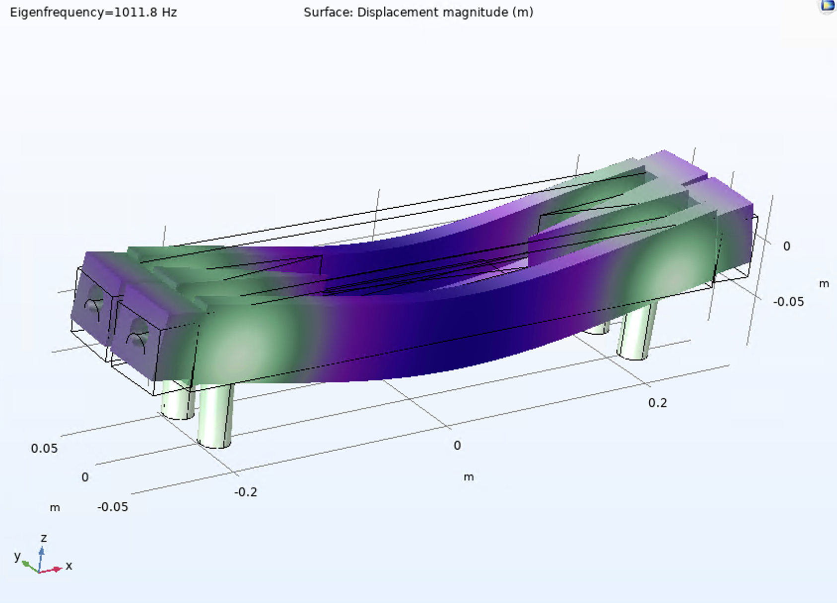
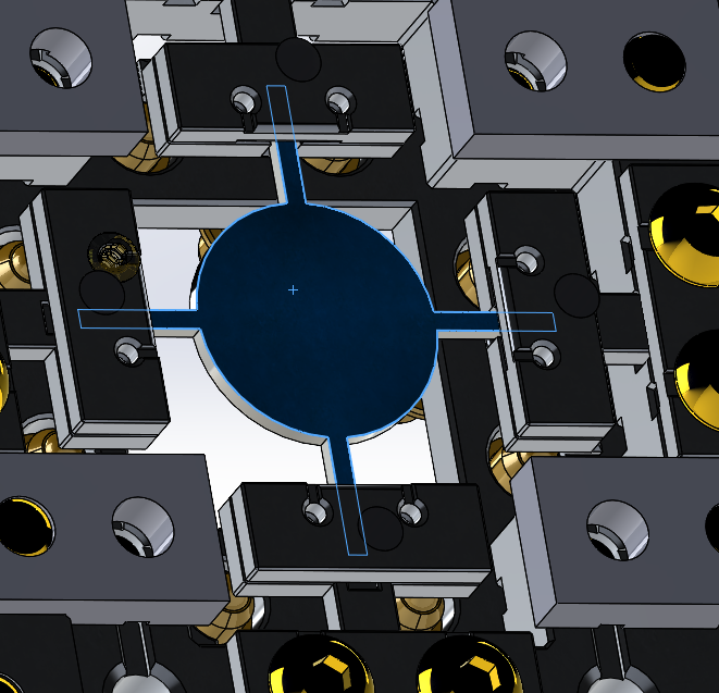
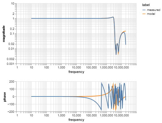
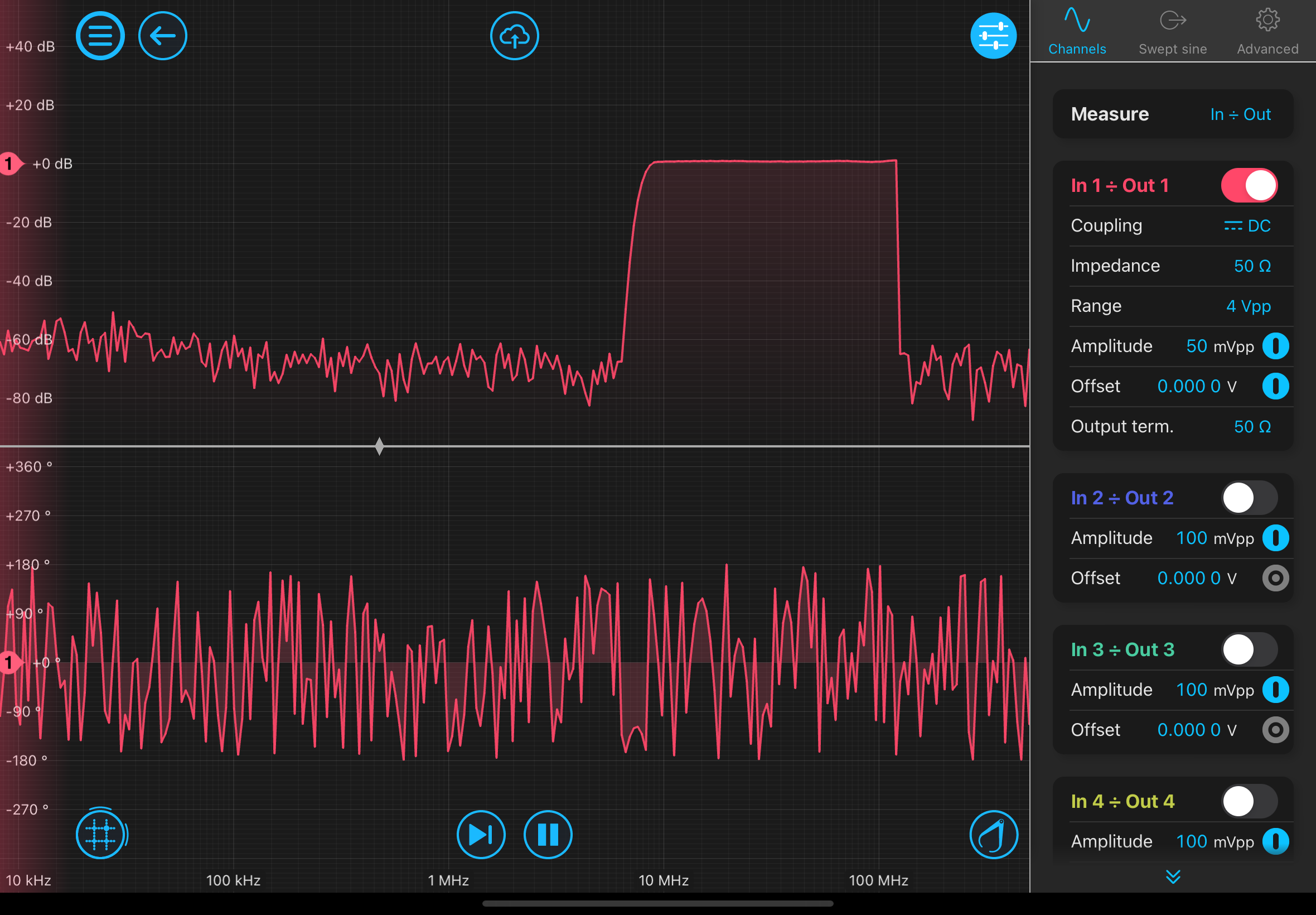
As followup to log post 11511, a transfer function of the band pass filter was taken and the delay calculated from the derivative of the phase. This gave a delay of 3.1 microseconds, in agreement with the pulse timing measurement.
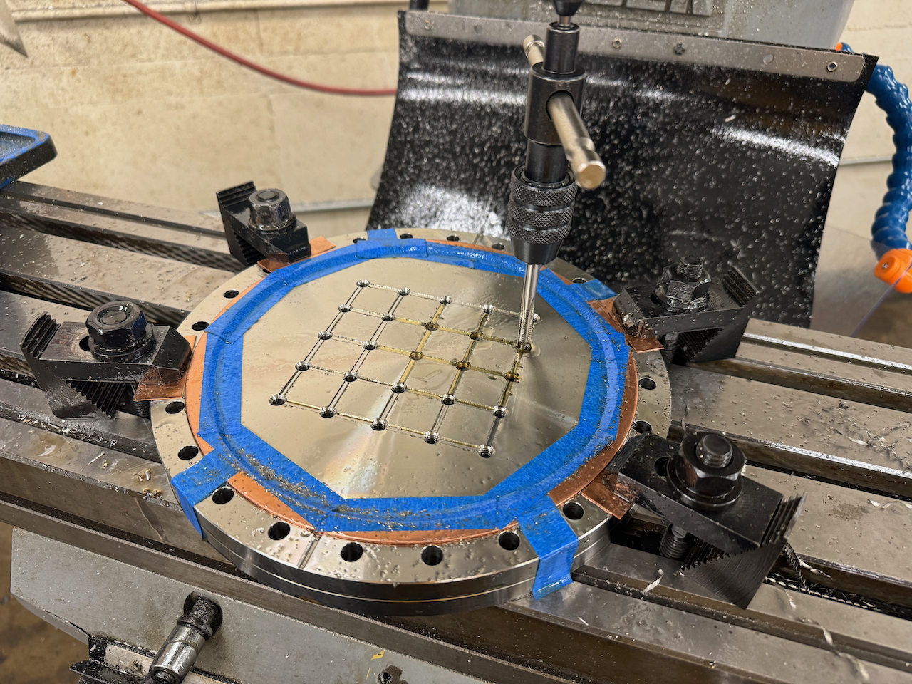
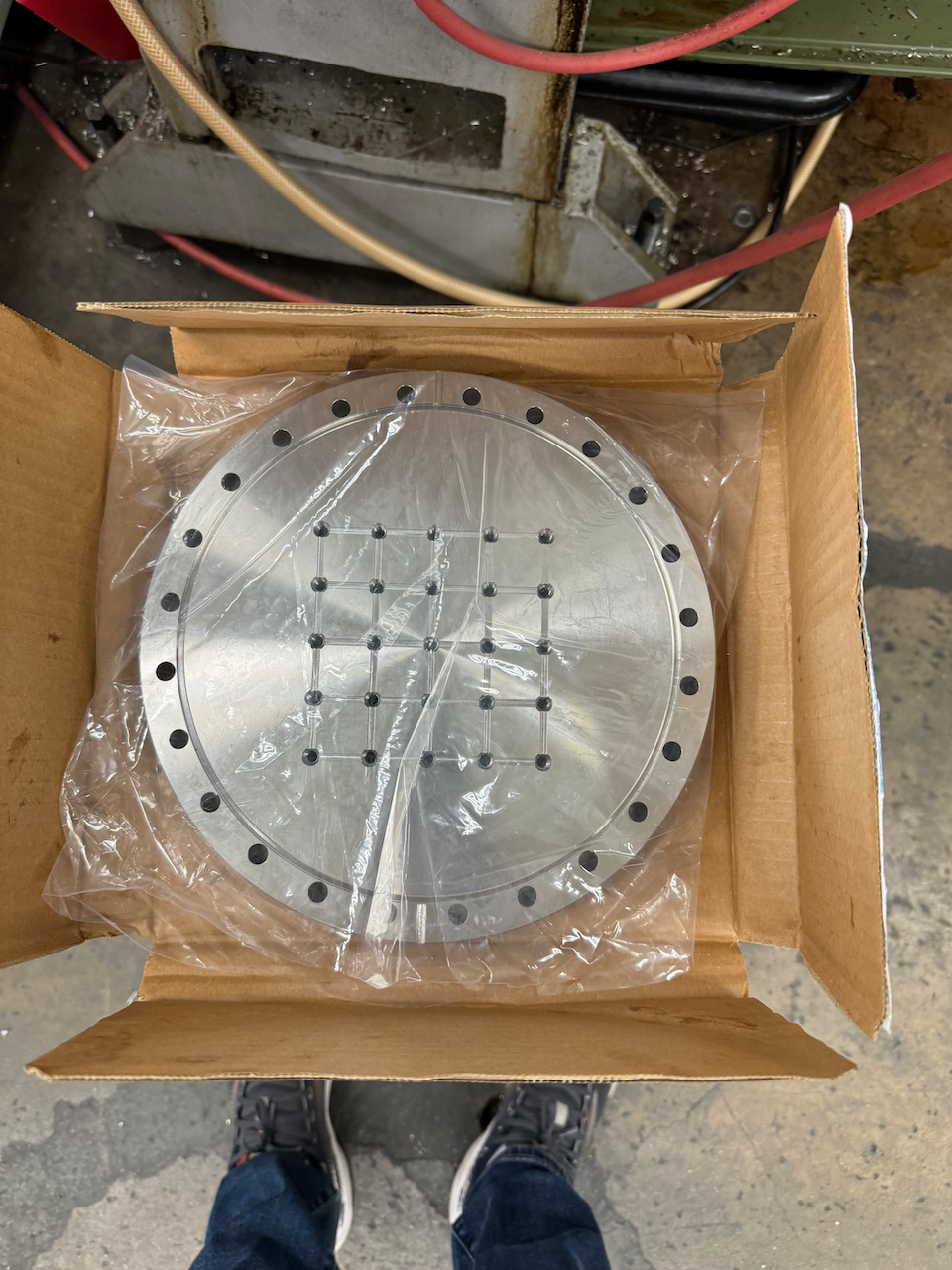
The two attatched pictures are of the band pass filter described in log post 11511.
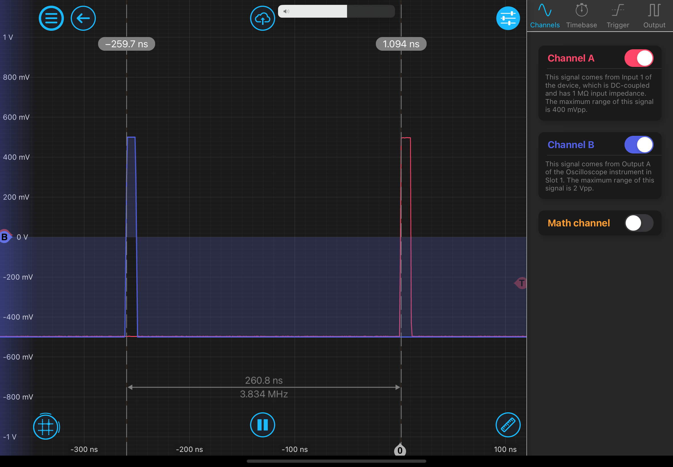
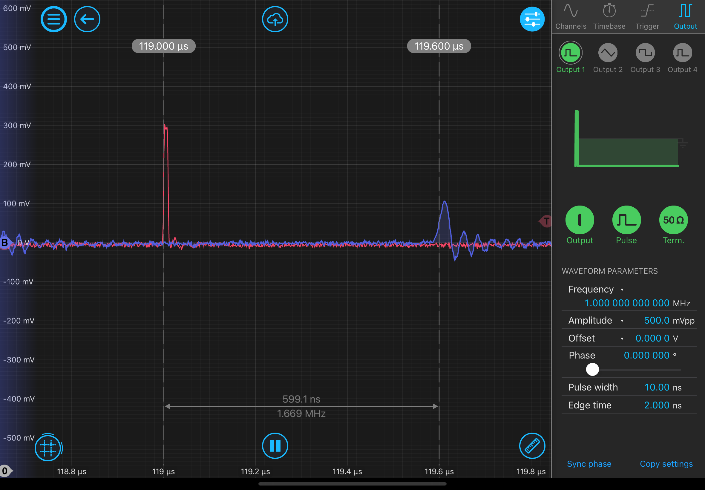
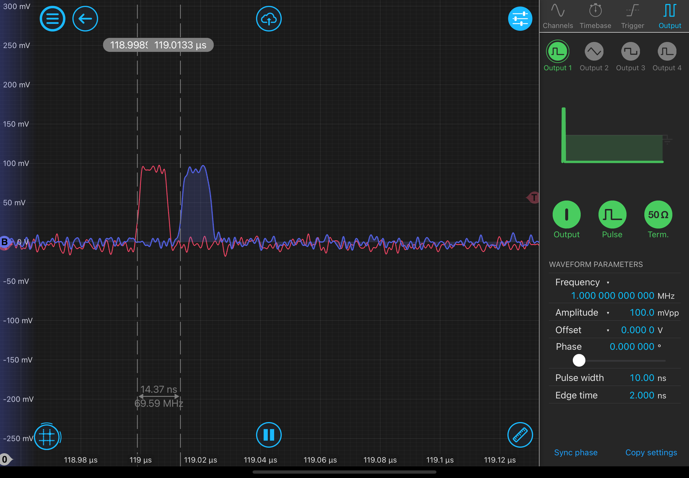
The amplitude of the signal going into the filter must be kept below 70mVpp to avoid strange effects. Sin waves in the passband with amplitudes of 50mVpp were observed to pass through the RFSoC without noticeable distortion.
Images attached to this report
Comments related to this report
Images attached to this comment