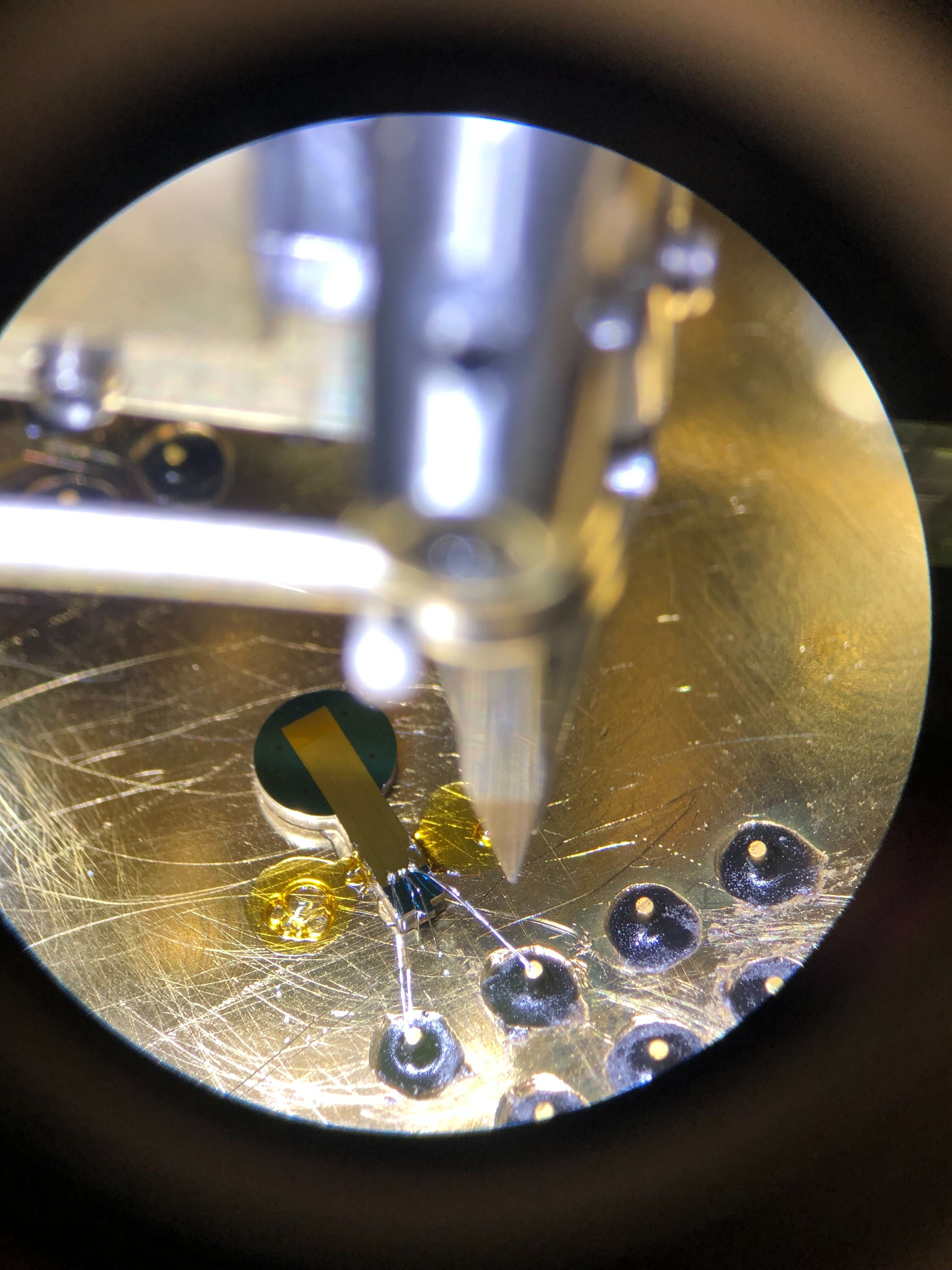
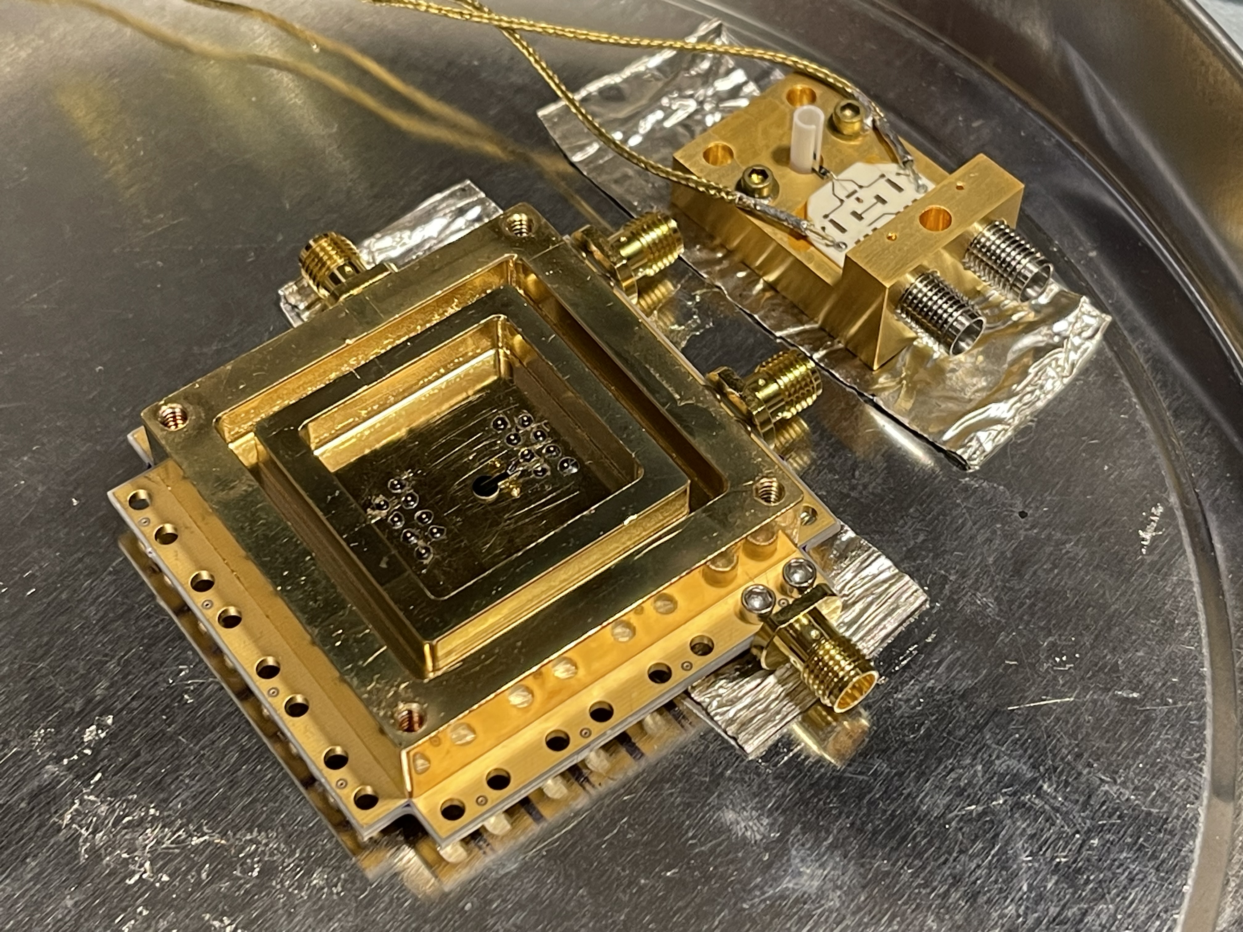
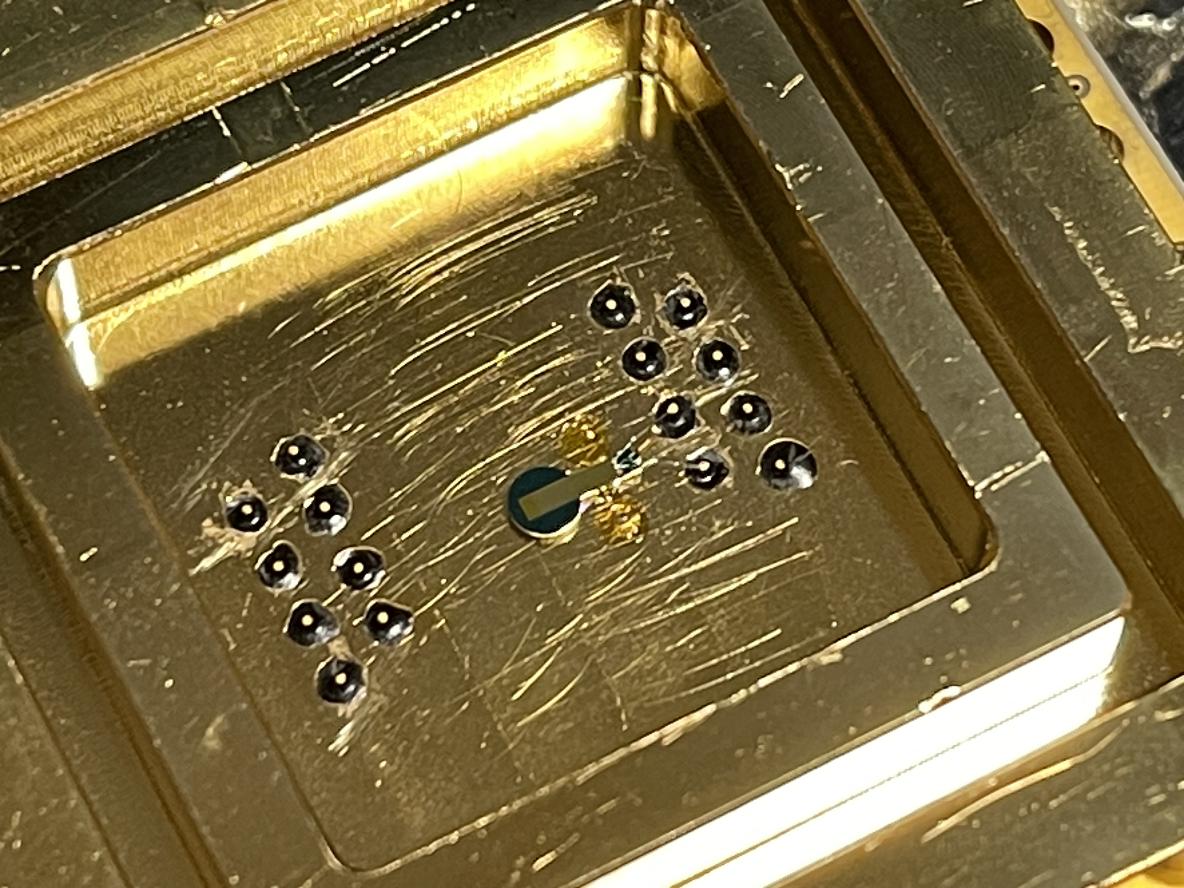
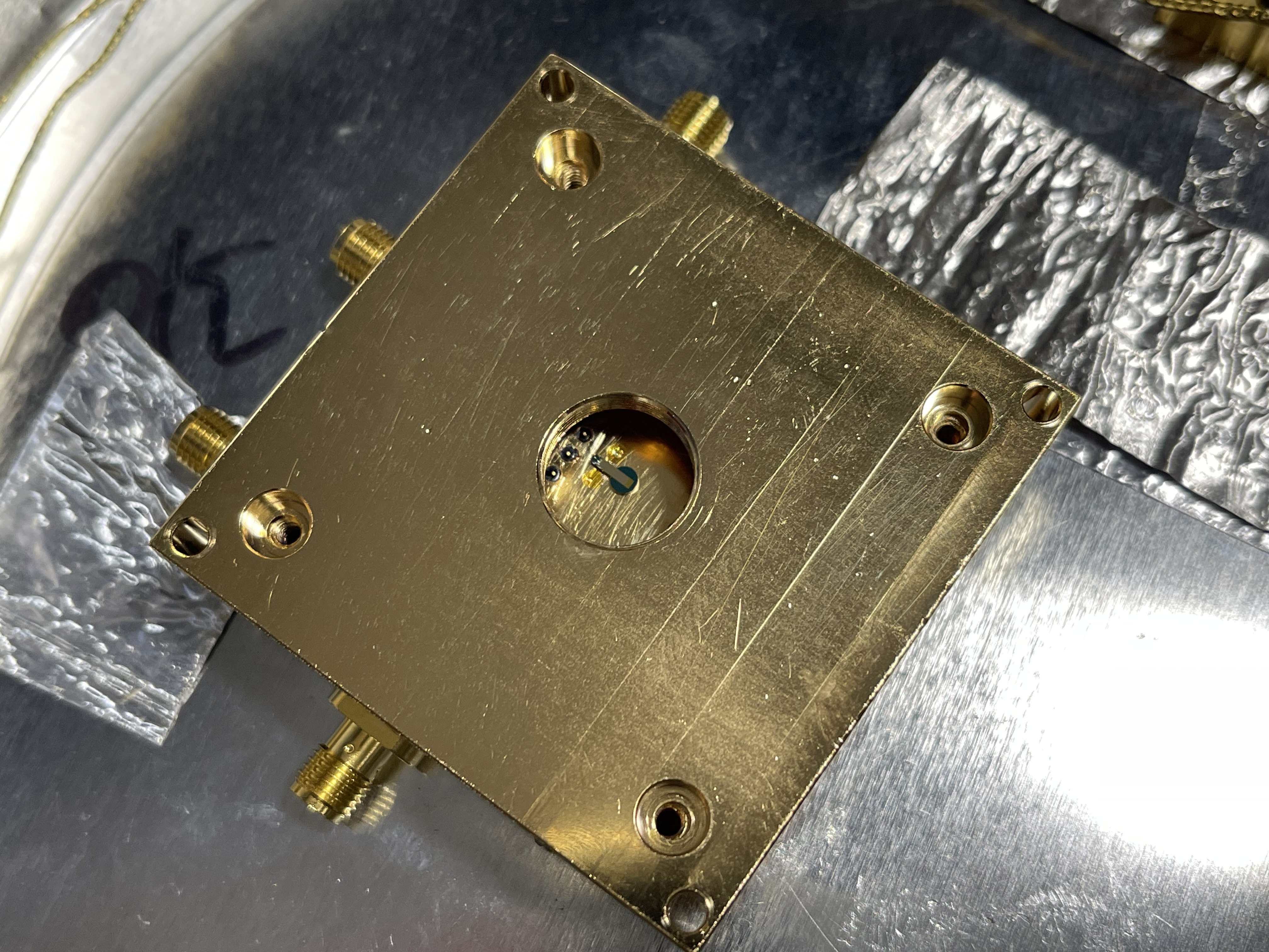
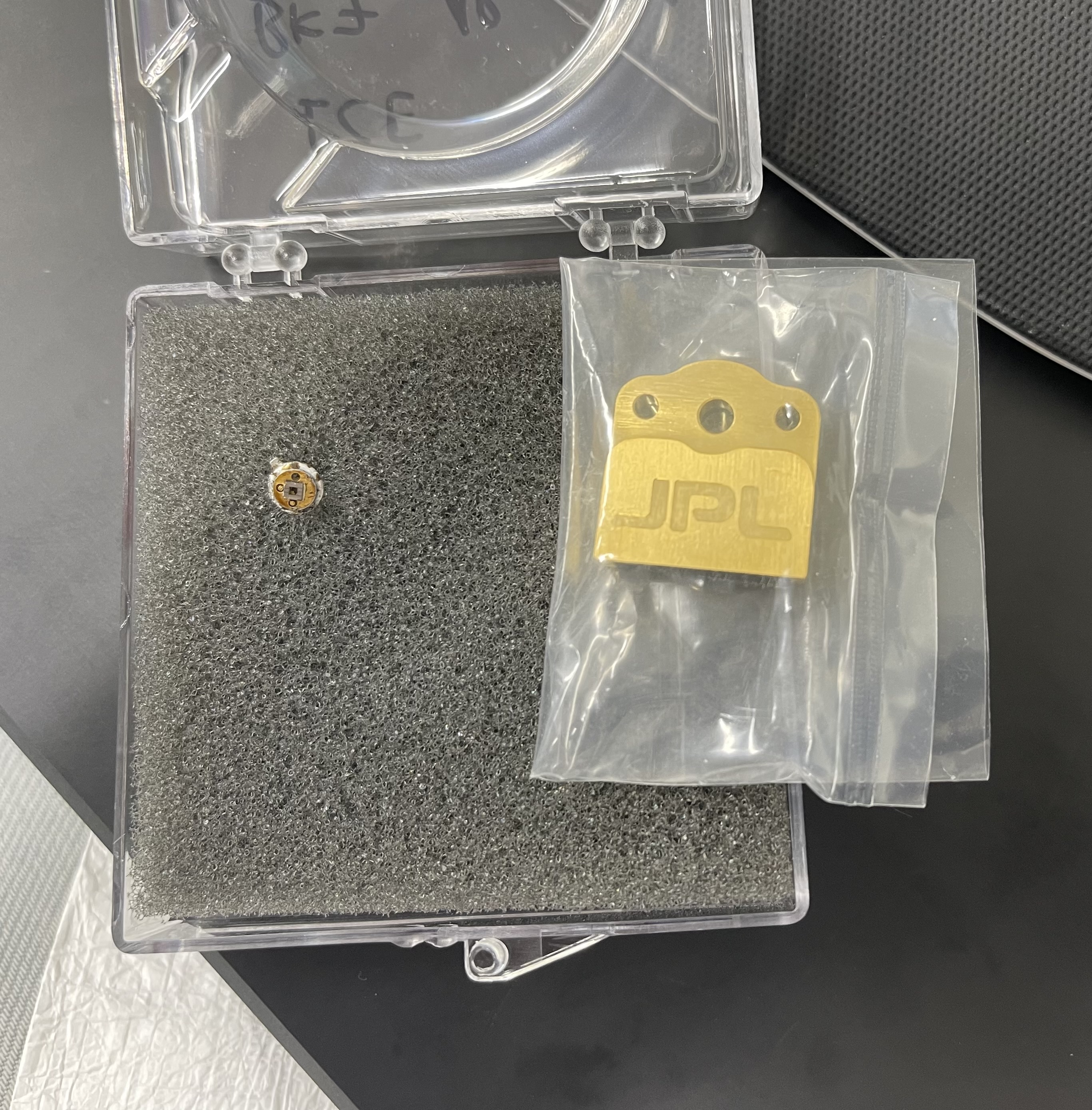
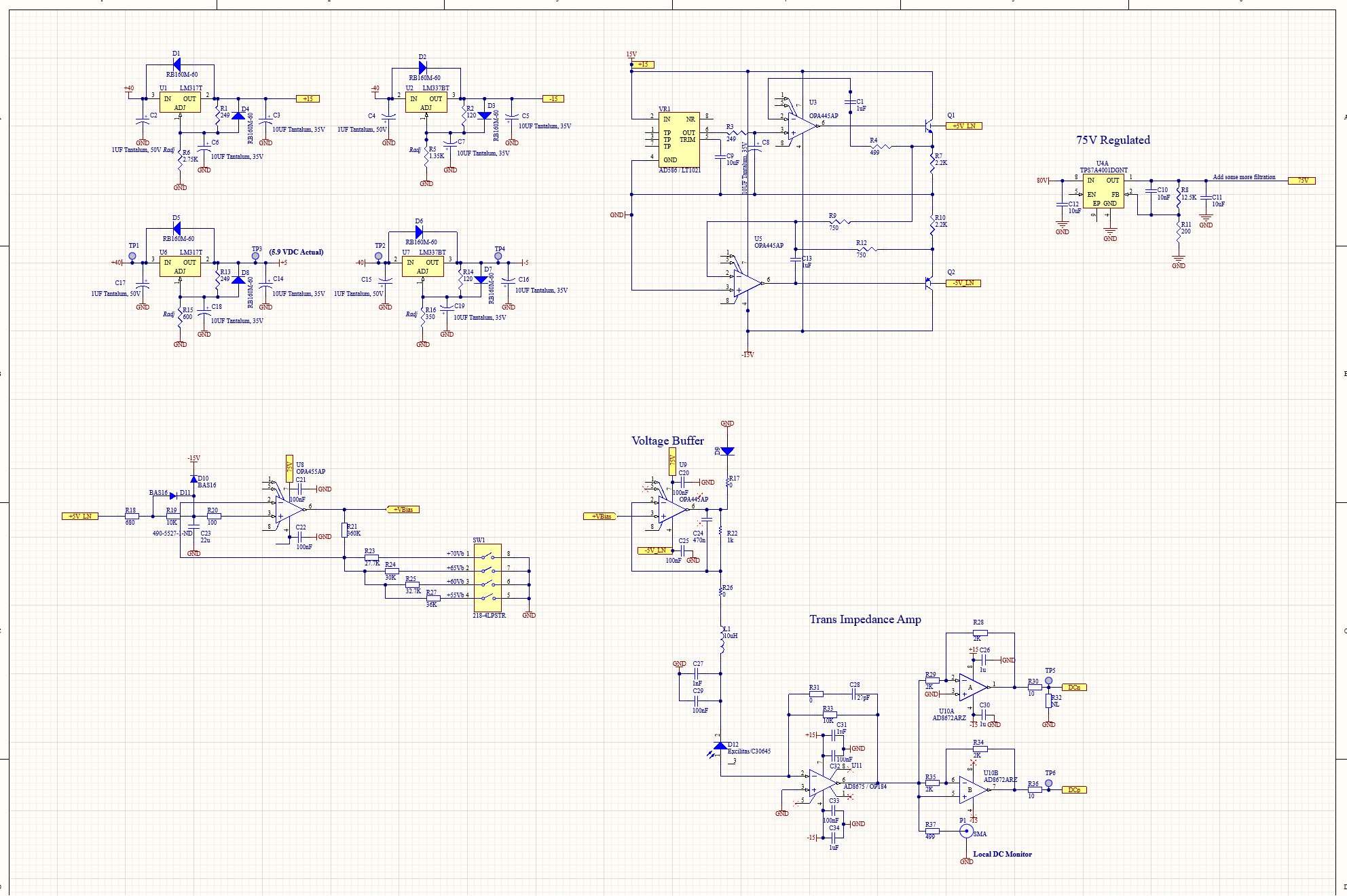
Boris and I have been working towards getting the SNSPD into the cryo chamber. There have been some hiccups as the chambers in Downs 123 have gone down recently, but we are looking toward taking an initial PCR curve next week (10/23/23) for the newly assembled SNSPD. See images 1-4 for the constructed SNSPD, wirebonded at JPL.
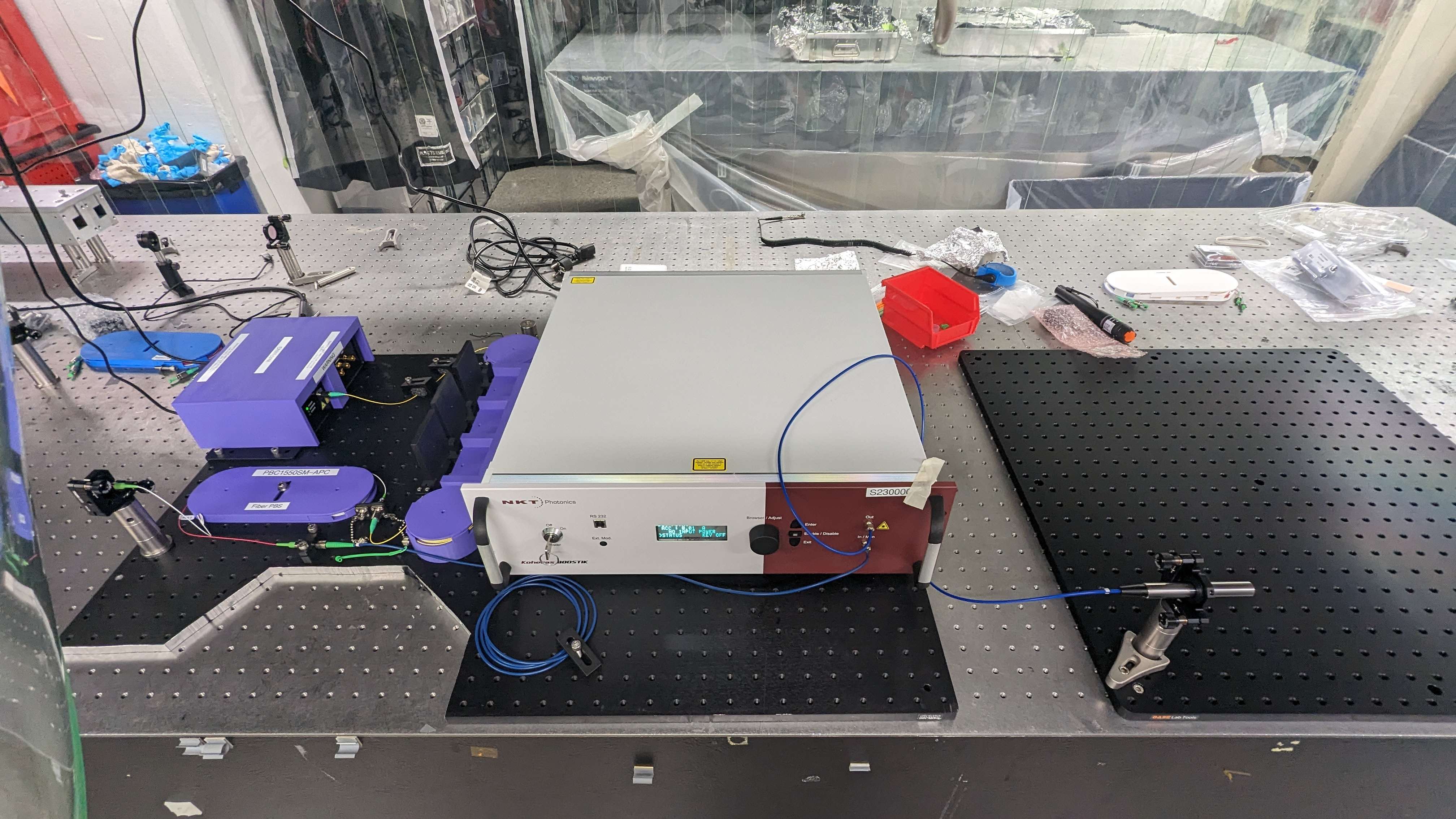
For the initial PCR curve on the SNSPD (to ensure it is working properly) we will use the top seen in image 3, which will allow us to place a fiber directly above the SNSPD for testing. Next, once we are happy with the results, we will go ahead and replace the top with a dark box enclosure to test the SNSPD performance on dark counts while completelty enclosed in the cryo-chamber.
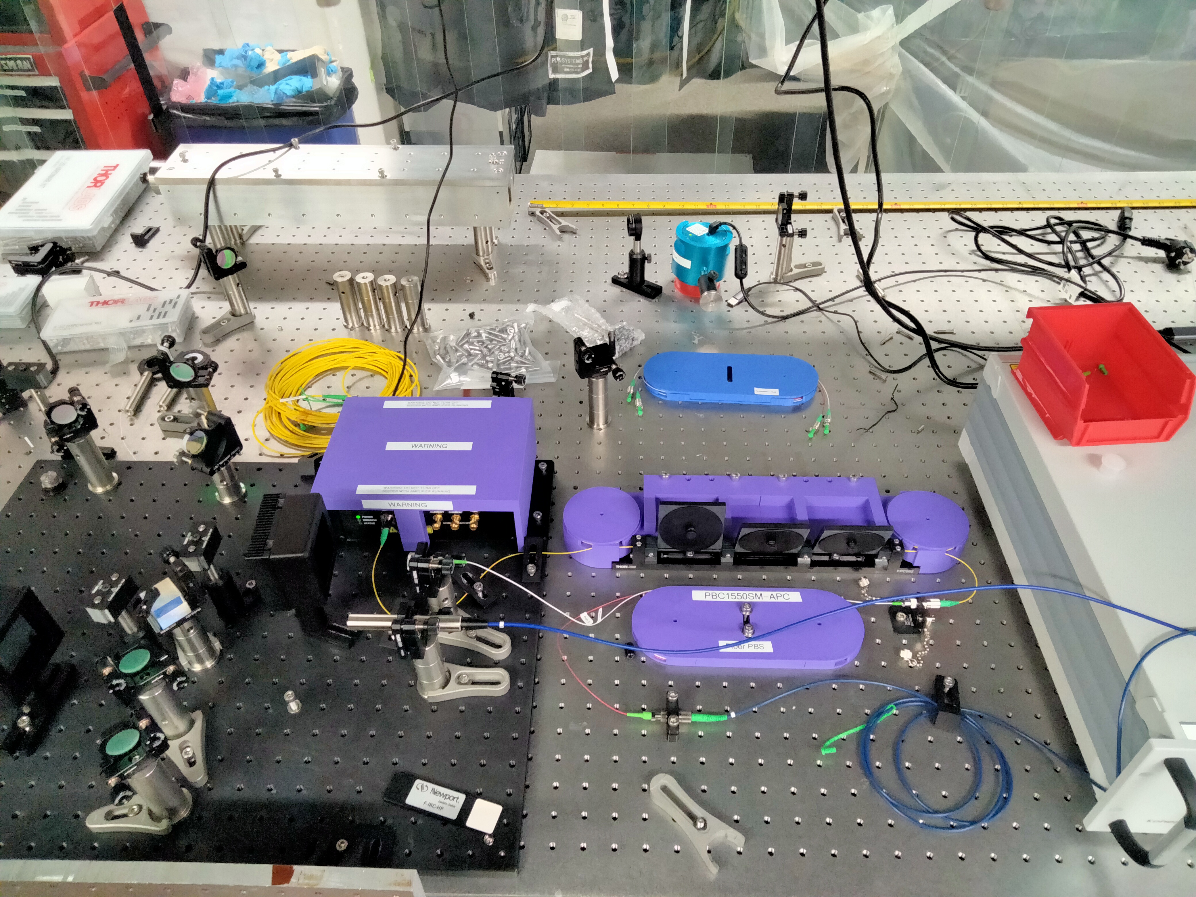
Finally, we will be testing the SNSPD's thermal response to radiation using a thermal source (axetris - EMIRS50 AT06V BR25M, attachment 7) and the setup seen in image 5. This setup will consist of the voltage controlled thermal source being placed approximately 1 mm away from the fiber tip allowing for complete exposure. The remaining fiber will be encapsulated in a brass tubing leading to the SNSPD. The setup utilizes thorlabs SM05 tubes and brass optic spacers to allow the thermal source to be held closely to the fiber. See image 6 for a real image of this thermal source.
We will be ordering these parts soon and assembling in the coming weeks.


