[Briana, Ian, Torrey]
Probe measurements again:
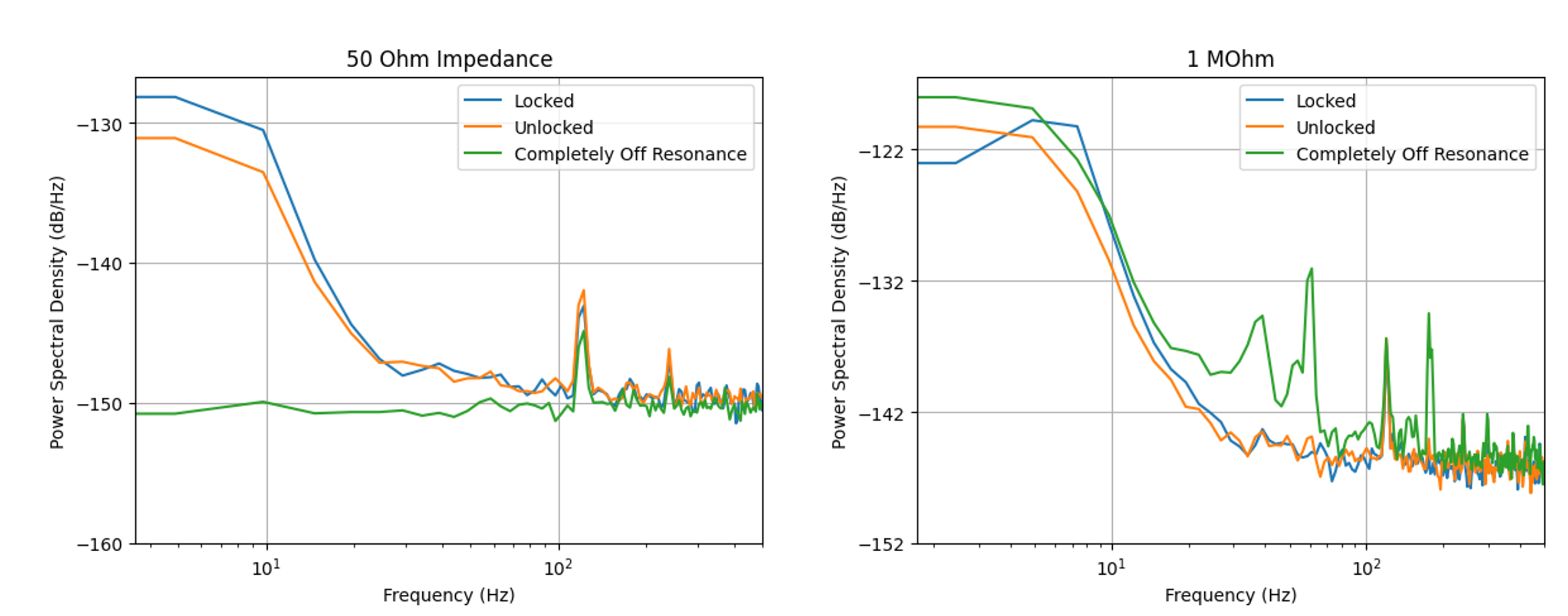
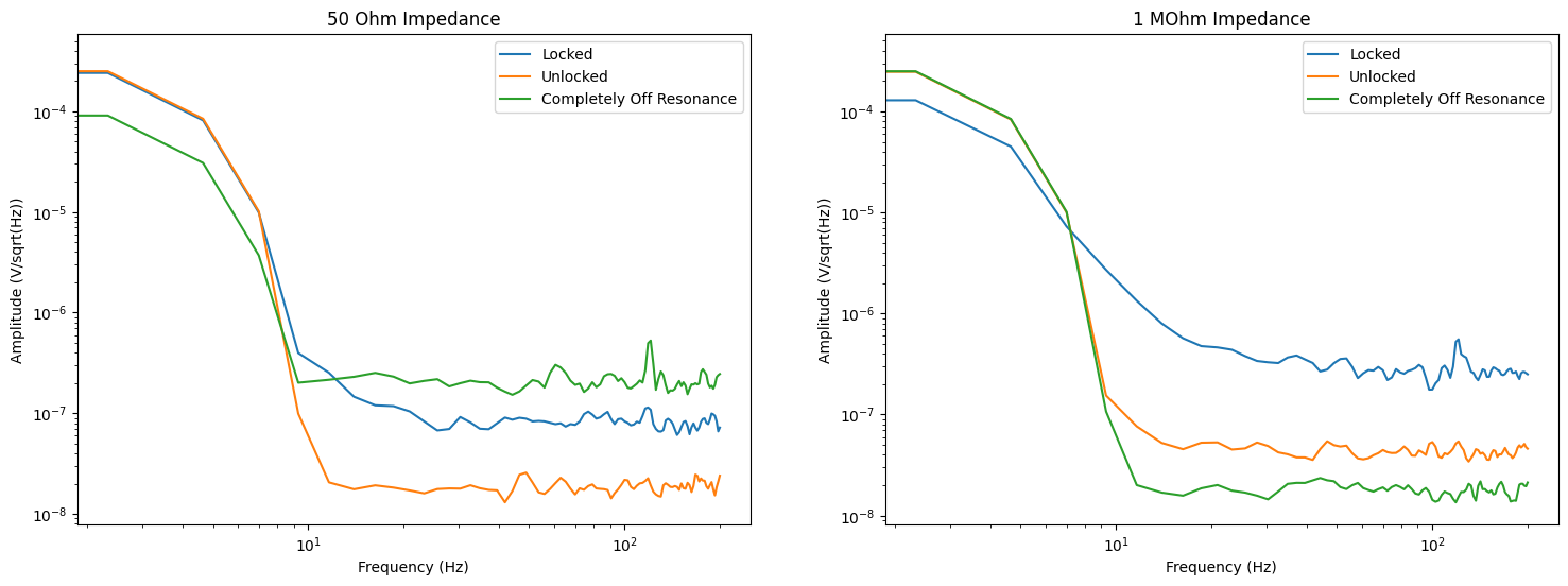
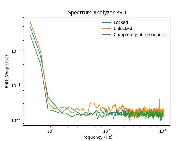
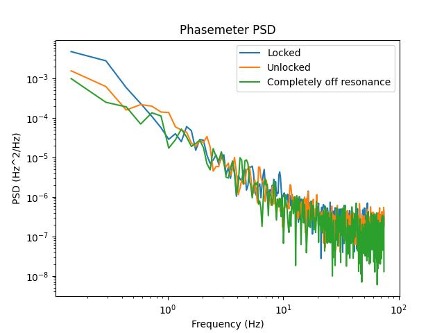
Retook spectra with just the probe to compare the results from using the matplotlib psd function (will switch to numpy), shown here probe_psd_python.png, and the Moku spectrum analyzer, shown here: probe_psd_moku.png. Data was taken for the photodetector input Moku channel at 50 Ohm impedance and 1 MOhm impedance to test at "different gains," although this does not really affect digitization noise since the signal would have already been digitized upon reaching the Moku- changing gain would have to happen before the Moku entirely. Regardless, the units of the y-axis are different between these two images but the order of which has the highest to lowest noise should be the same. However, the Moku spectrum analyzer provides less resolution so the shapes (especially <10 Hz) are not easily comparable and I am generally having a hard time trusting the spectrum analyzer. The general order of highest to lowest noise is somewhat consistent at <10 Hz. For 50 Ohms, after moving the offset of the temperature controller completely off the temperature at which the absorption occurs, we somehow see less noise compared to when the laser is locked, which is very bizarre. It is possible that the laser may just become very stable at that random temperature that I detuned to. Also, the noise level for the spectrum analyzer at higher frequencies is offset in the spectrum analyzer, in contrast to the post-processing method which shows what we would expect: noise at higher frequencies is the same across all three cases because the actuator does not implement control at those frequencies. I'm not sure why the spectrum analyzer behaves like this.
Attempts to amplify signal: We want to amplify the signal to reduce effects of bit noise, even though we amplify other noise in the process. Dominating bit noise could be one cause of these confusing noise spectra.
Built tank circuit for the EOM to enhance the error signal as much as possible. Resonant EOM seems to occur at 123 MHz after optimizing phase shift for different modulation frequencies. The EOM has capacitance of 14 picofarads. For a resonant frequency of 122.9 MHz, this means we get an inductance of L = (1/2pi f)^2 / C ~ 119 nano Henries. The resulting tank circuit did not work: touching the BNC cables even slightly changed the error signal significantly, and the signal was not amplified- in fact, the amplitude was larger without the tank circuit. We will proceed without the tank circuit for current time constraints. Connections are fine in the circuit (tested with the silver remote box), but maybe the components/connections are not secure and thus extremely sensitive to the environment/movement.
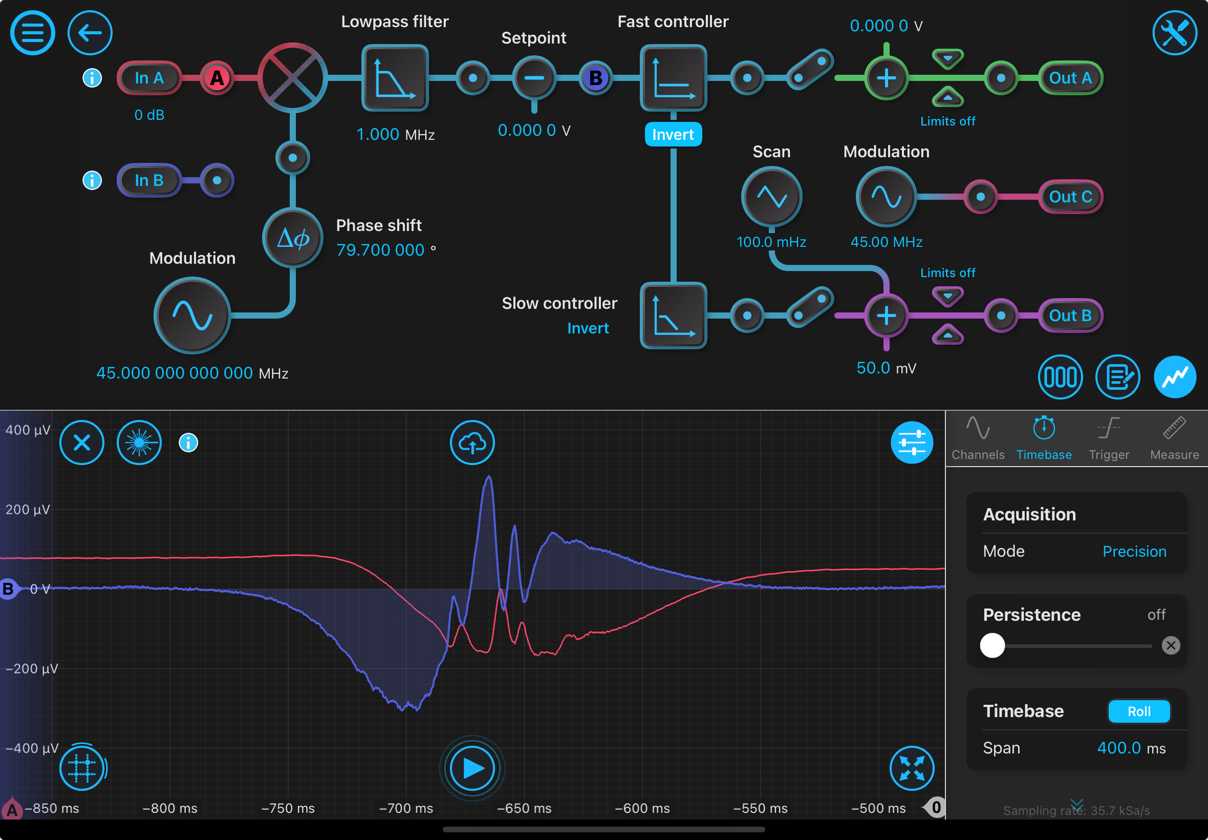
We want to amplify the light passing through the vapor cell before reaching the Moku (i.e. getting digitized), so we tried adding a low noise amplifier (LNA). I stole the one from the new lab which somehow works better (less noisy signal) than the one in the beige cabinet in B102 even at the same settings. However, amplifying the signal (with lowpass filter on the LNA set to the highest setting of 1 MHz) caused the error signal to become <20 microvolts in amplitude compared to the previous >400 microvolts in amplitude without the LNA, no matter how the modulation frequency/phase is tuned. The error signal also becomes a distorted symmetric shape. I think this is a filtering issue with the lowpassing. Although the photodetector signal from the temperature scan looks the same as without the LNA, maybe the modulation signal strength is not strong enough (the one getting mixed with the photodetector signal) to produce a significant amplitude for the error signal. Additionally, the error signal is very sensitive to moving the BNC cable to the EOM when connected to the LNA. Without the LNA, the error signal is not sensitive to BNC cable movement, so this is some issue with the LNA. Some of its specifications (from here) should also be considered when troubleshooting, although I don't think they are the sole reason for these problems: 1). the output type is a 100 Ohm BNC, so we might want a 100 Ohm BNC cable attached instead of a 50 Ohm (?) and 2). the input to the LNA must be between -0.4 and 0.4 V to get accurate readings (this is fine with our input signal, which usually doesn't even reach 200 mV). We are proceeding without the LNA for now. One idea to troubleshoot would be forking two outputs from the LNA into the Moku, one AC and one DC coupled. AC removes the DC offset so this coupling means that only AC signals will pass through, effectively acting as a lowpass filter. If the error signal is prominent in AC coupling, it could mean we just have an issue with the settings for modulation frequency/phase/low-pass filter in the Moku.
Pump:
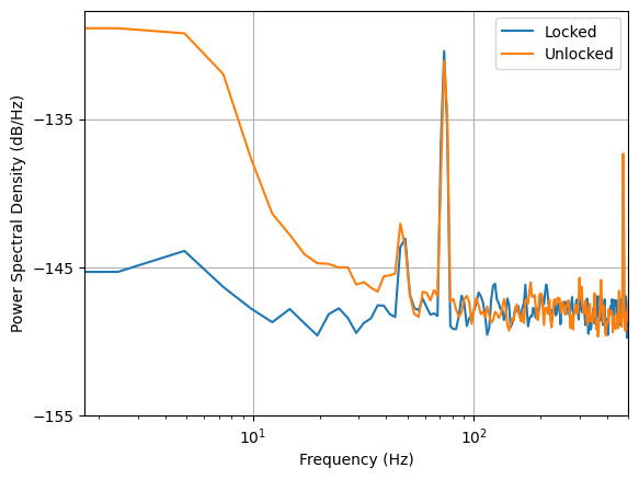
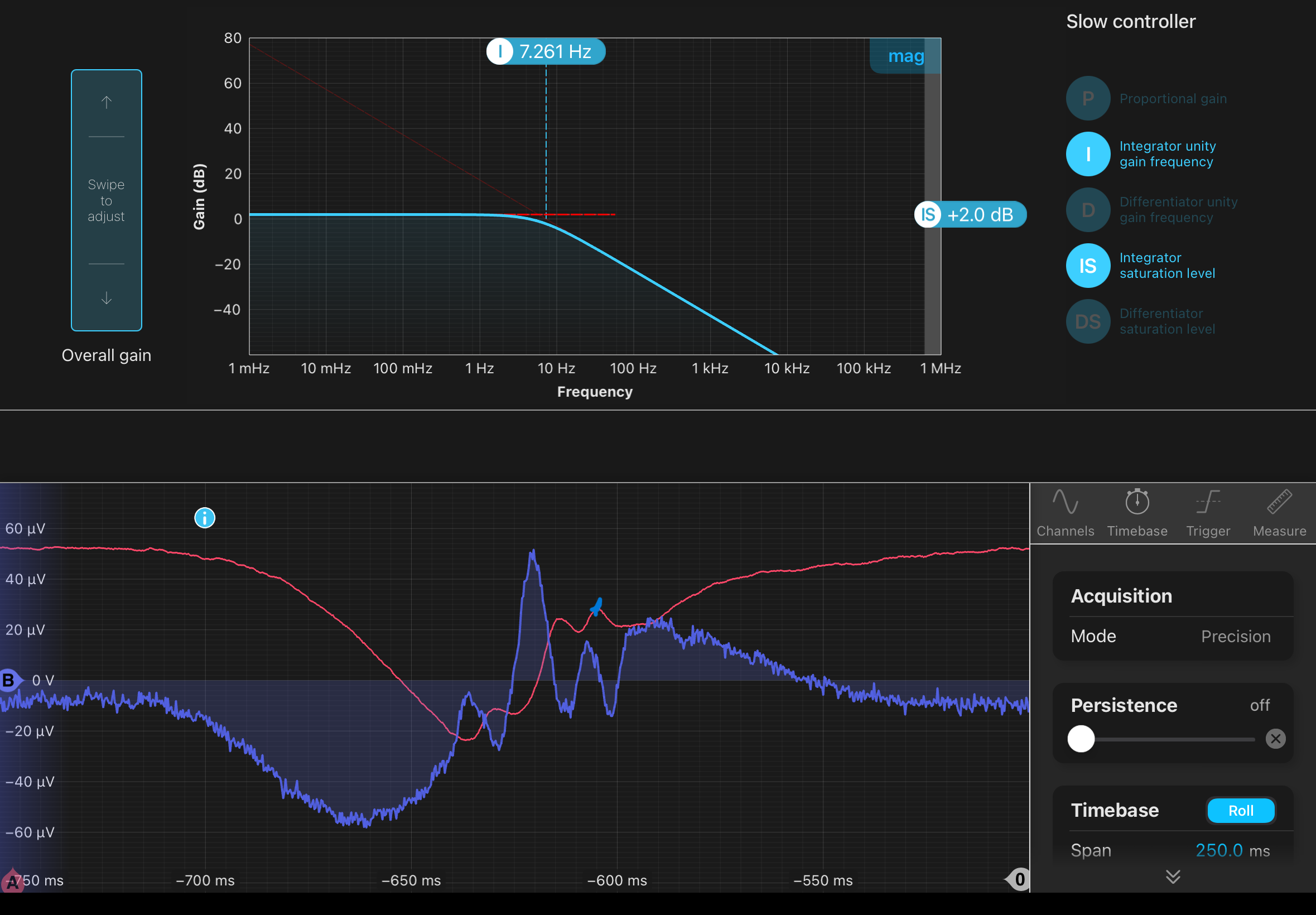
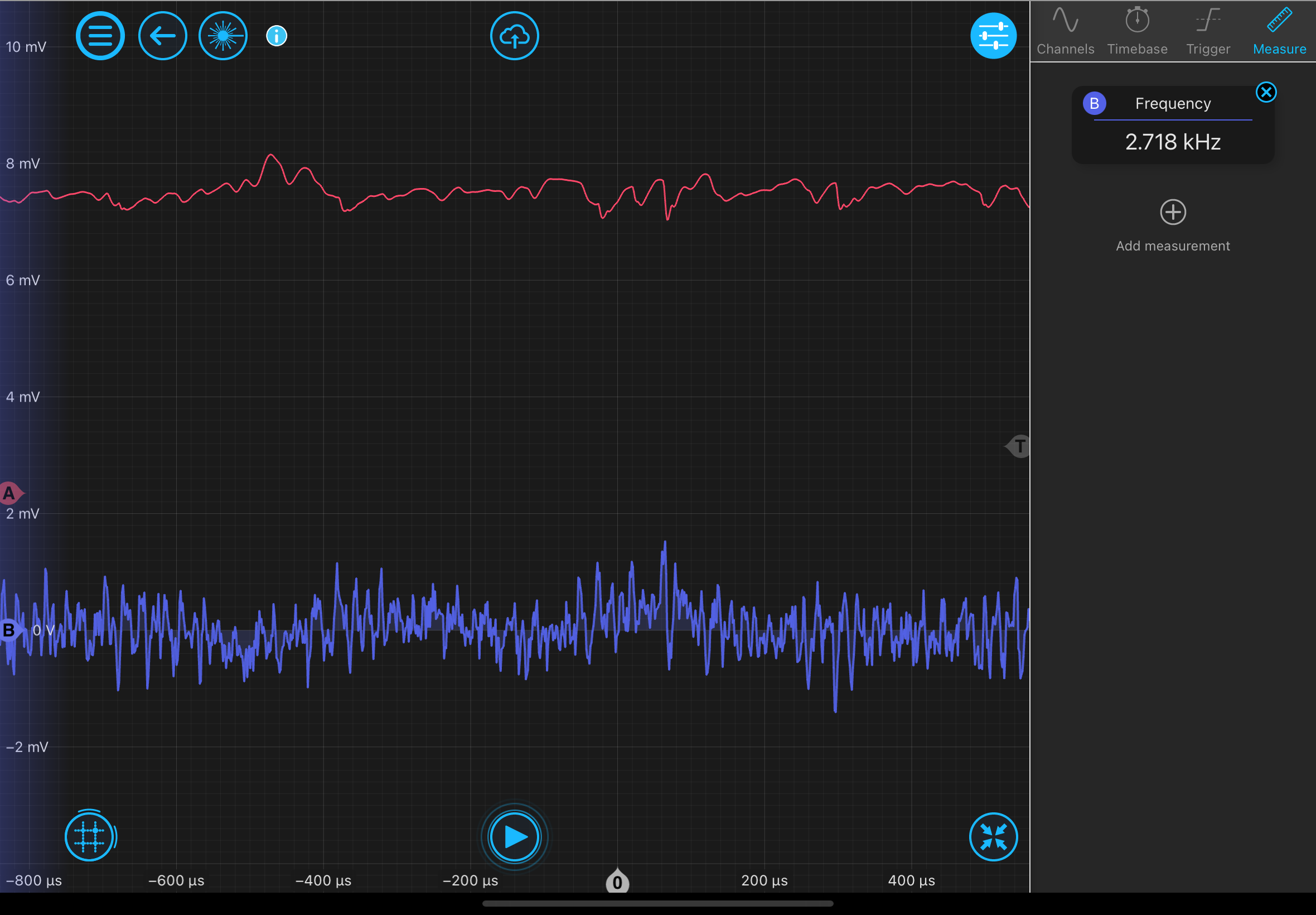
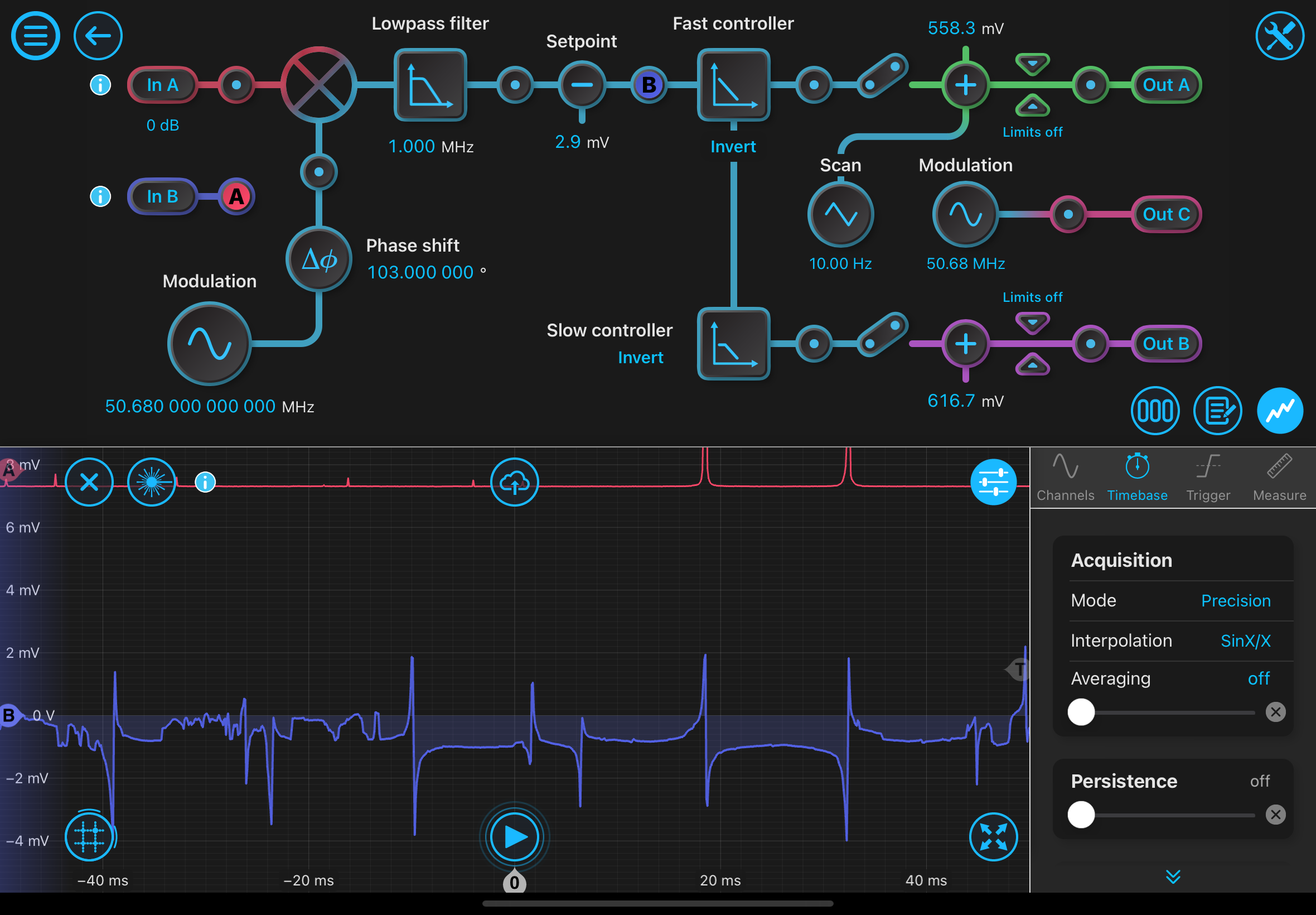
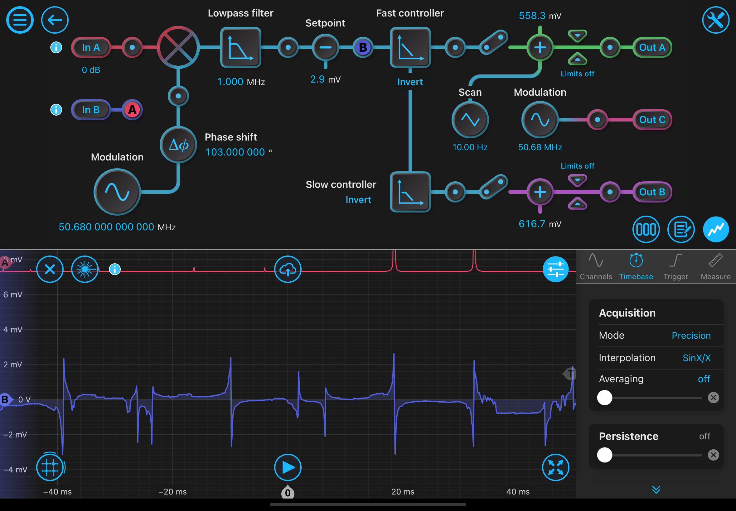
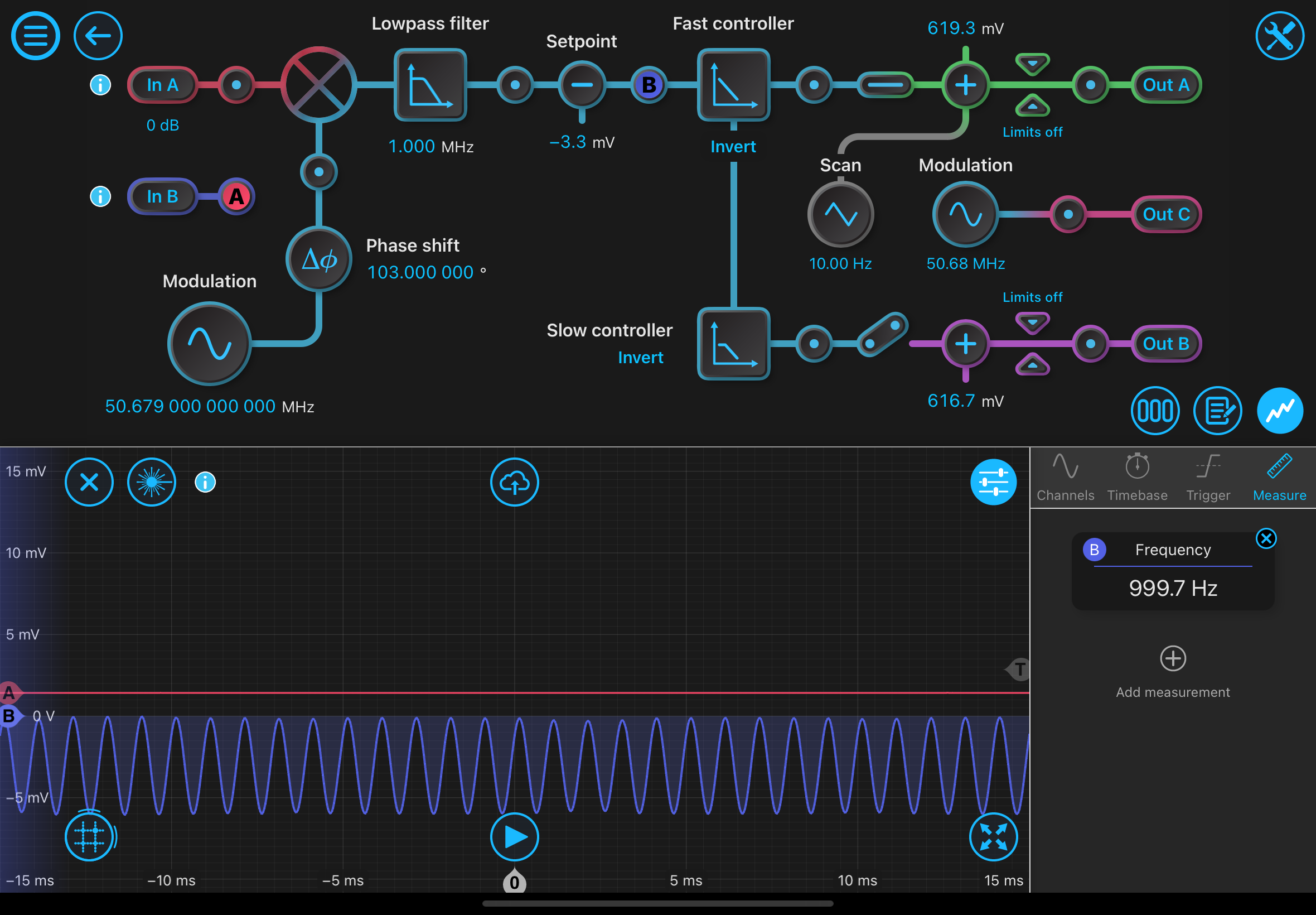
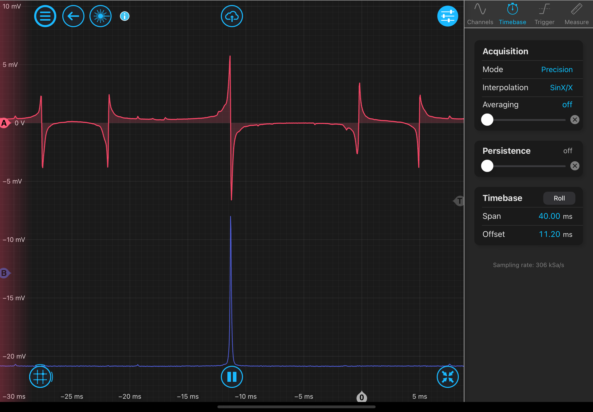
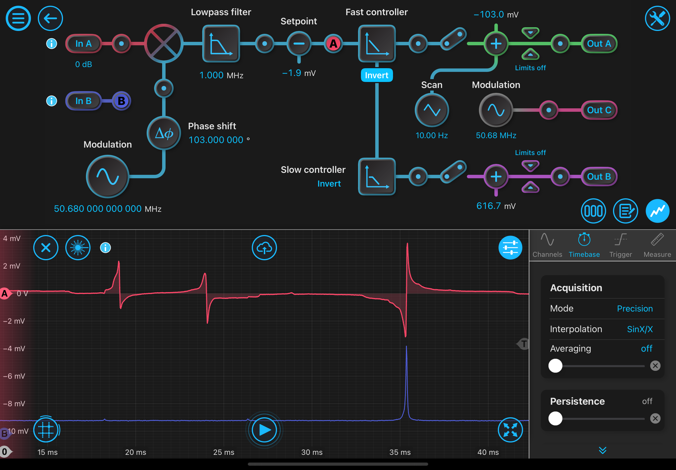
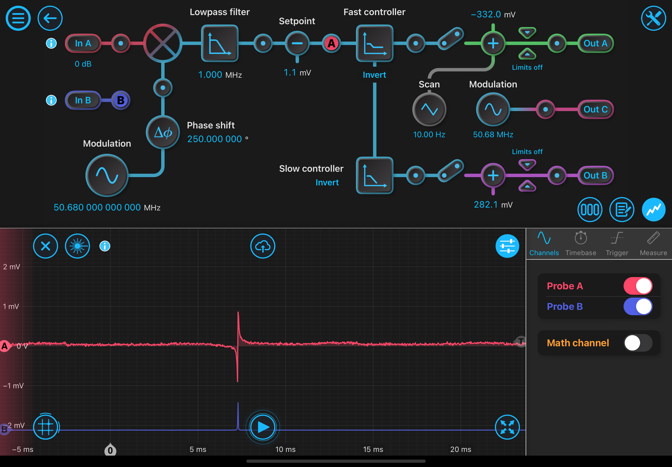
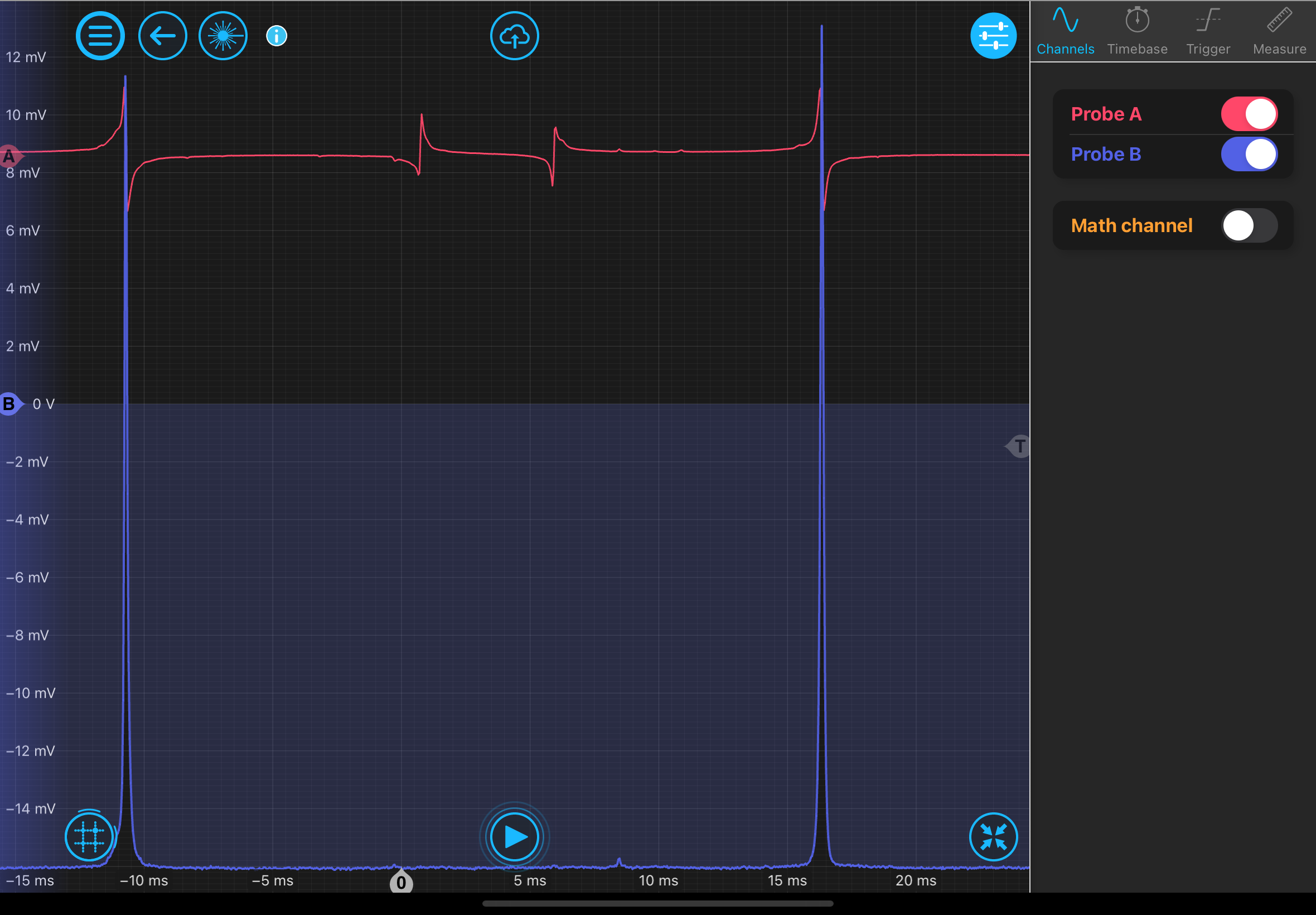
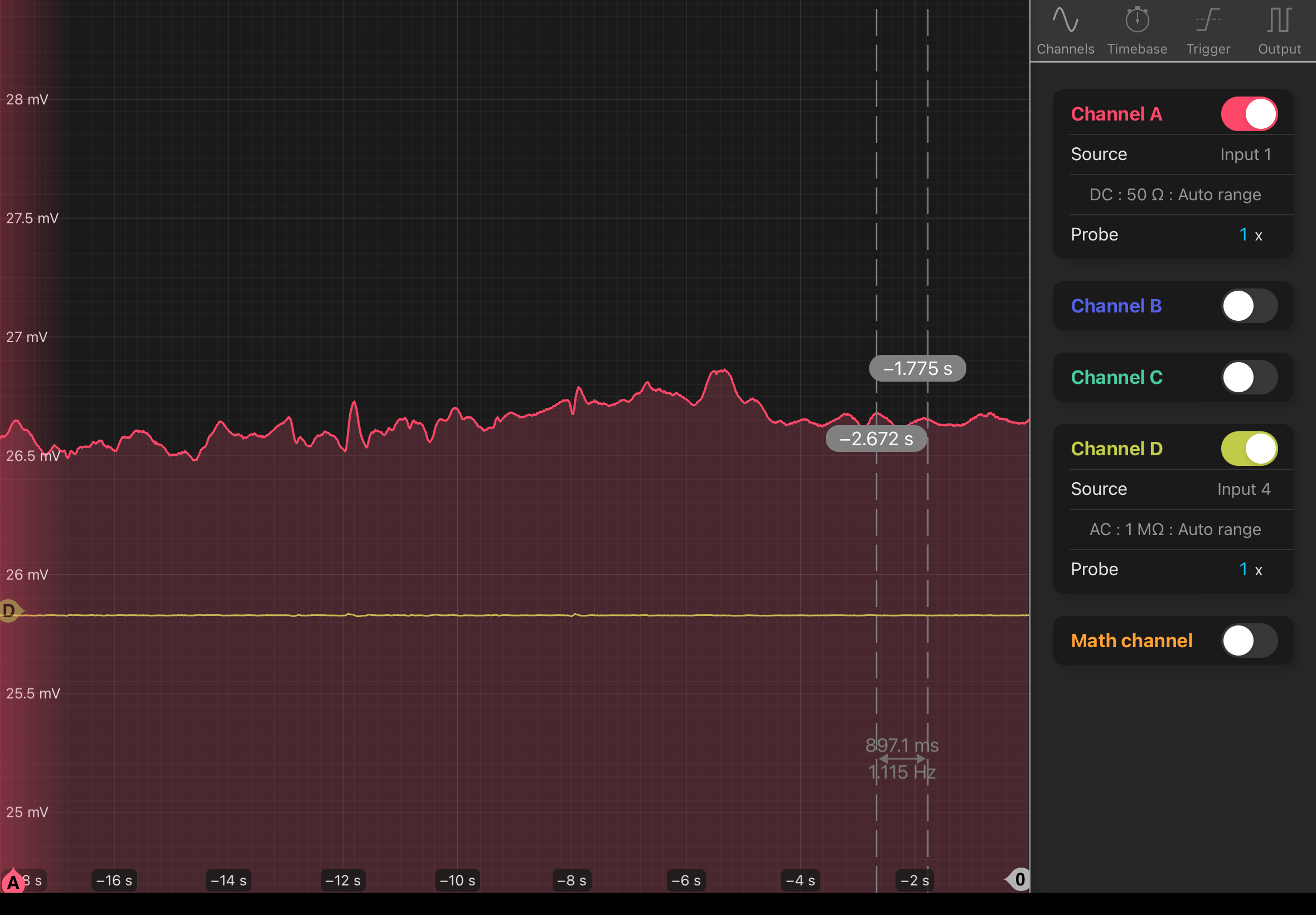
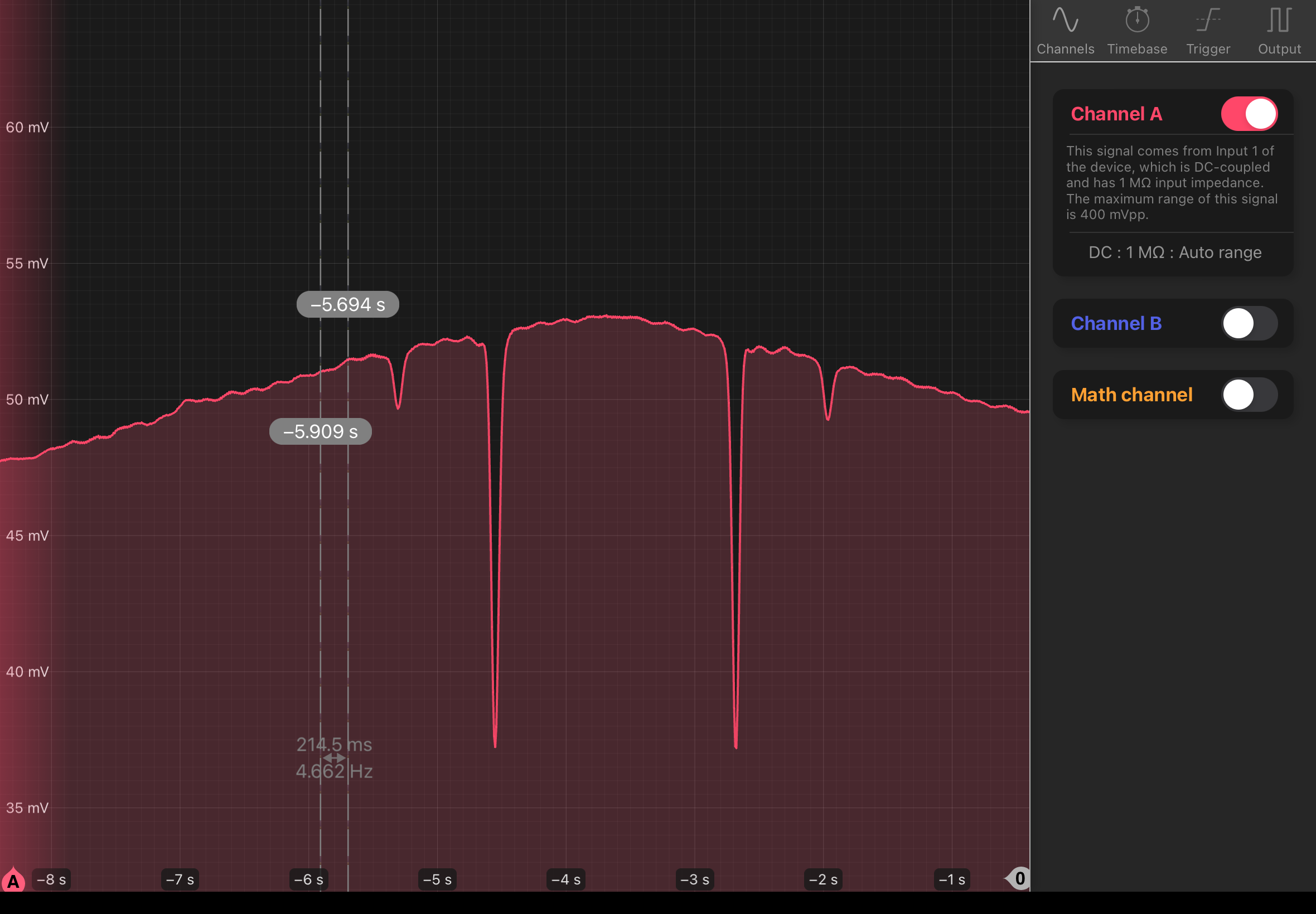
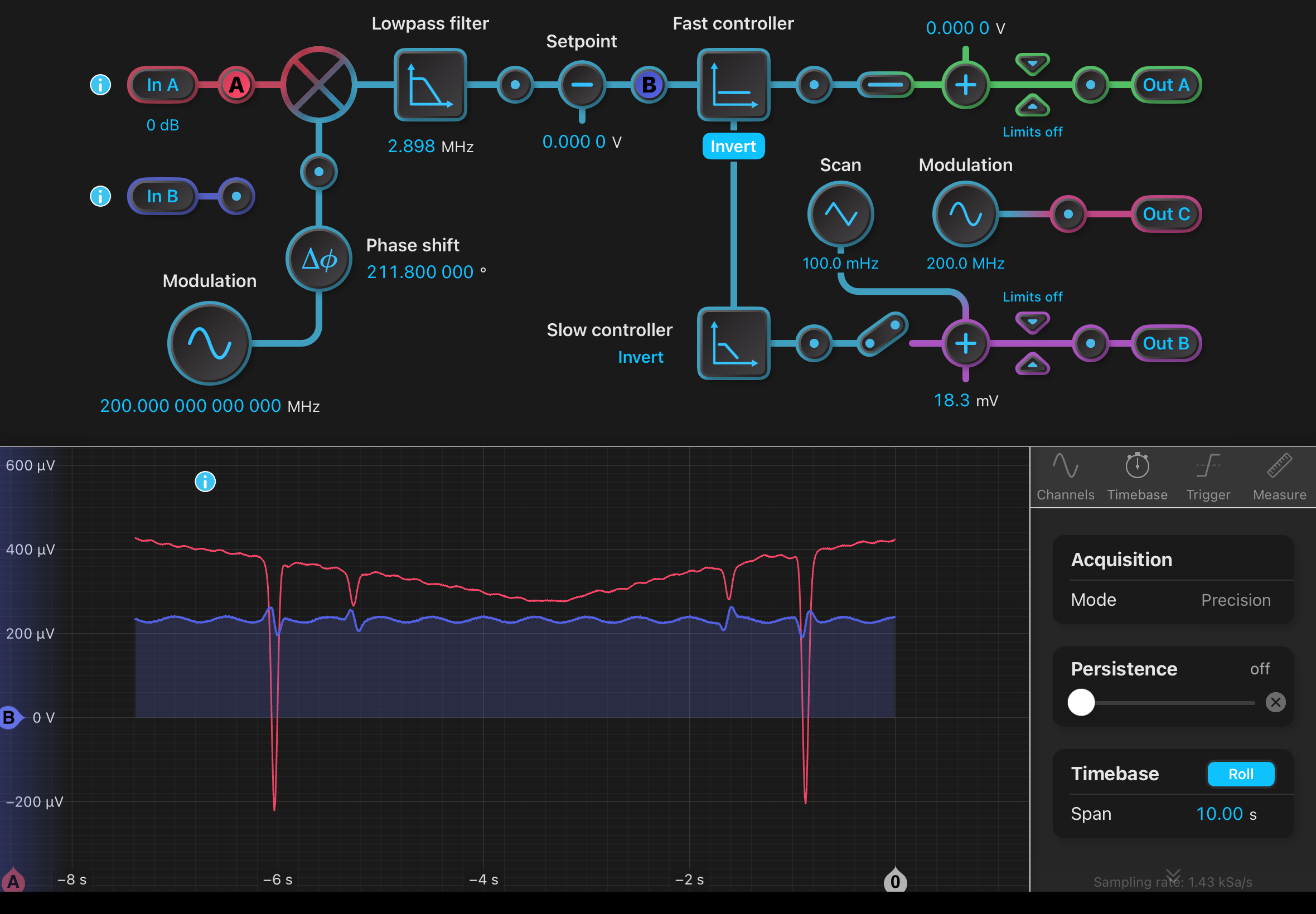
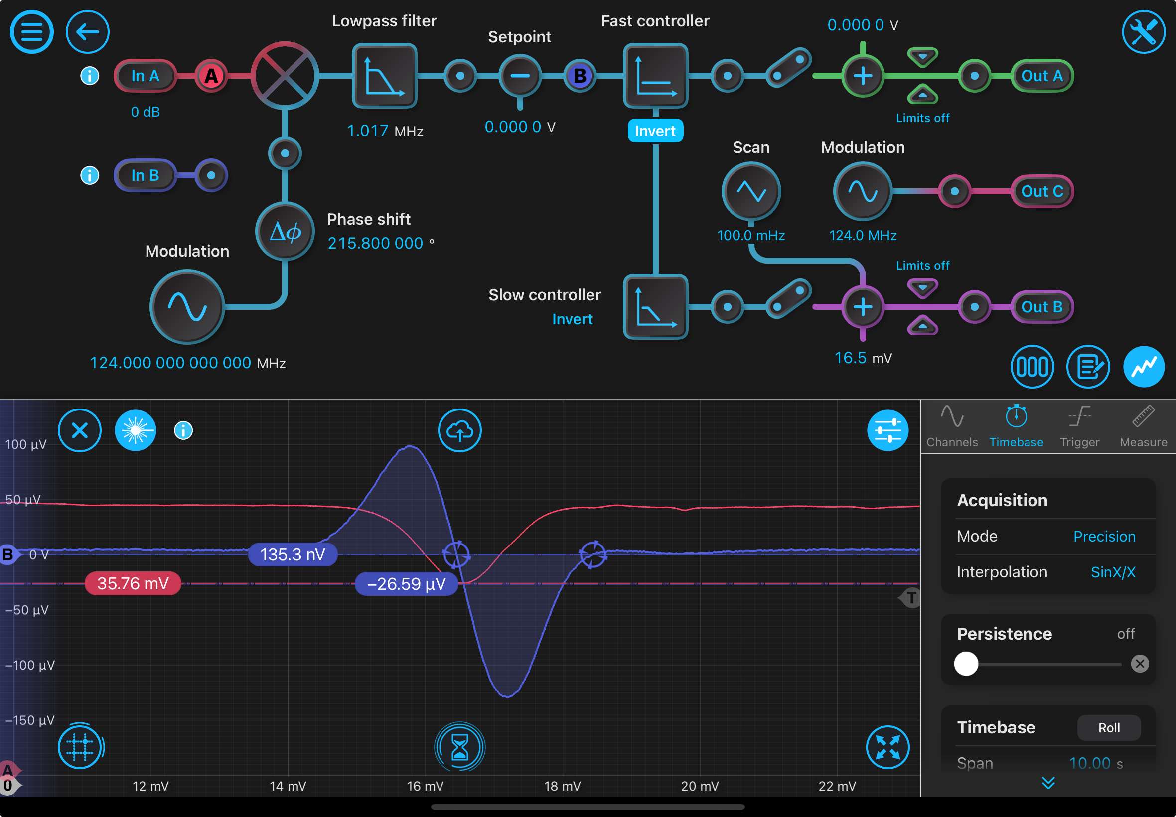
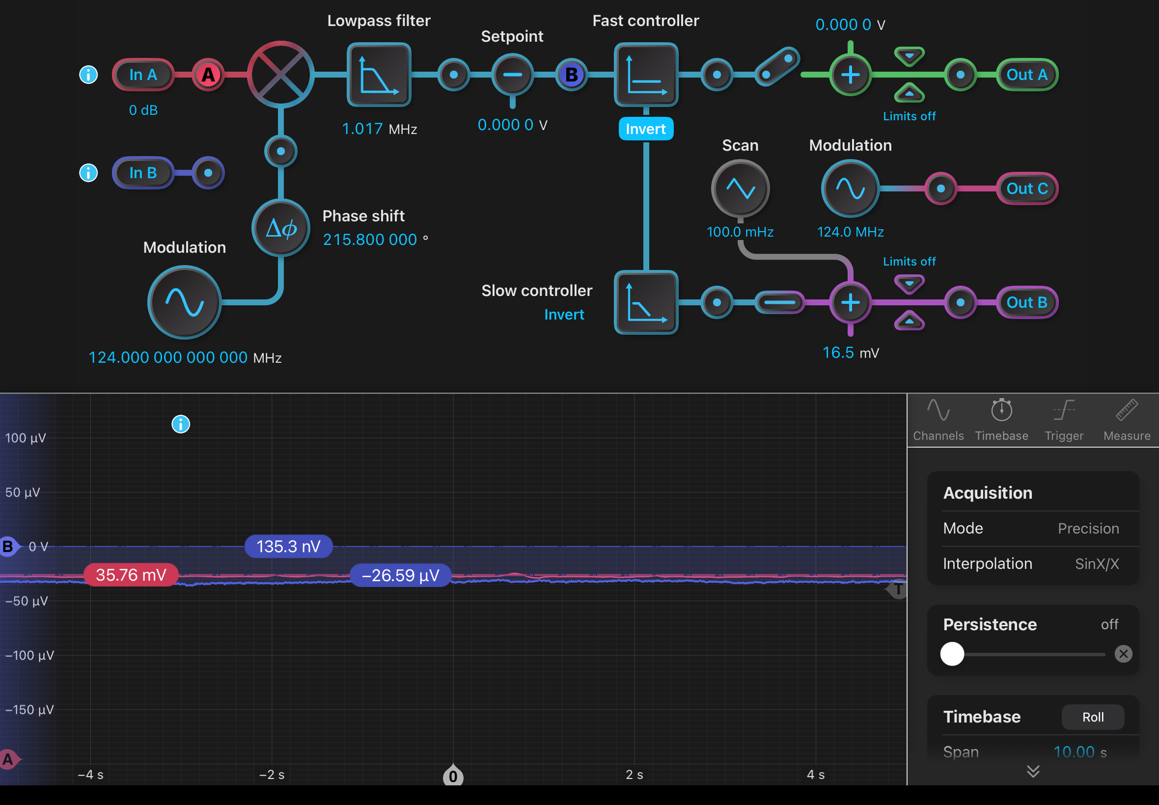
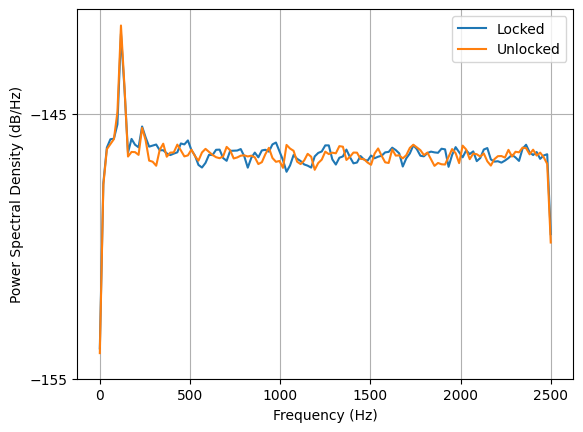
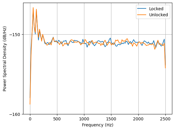
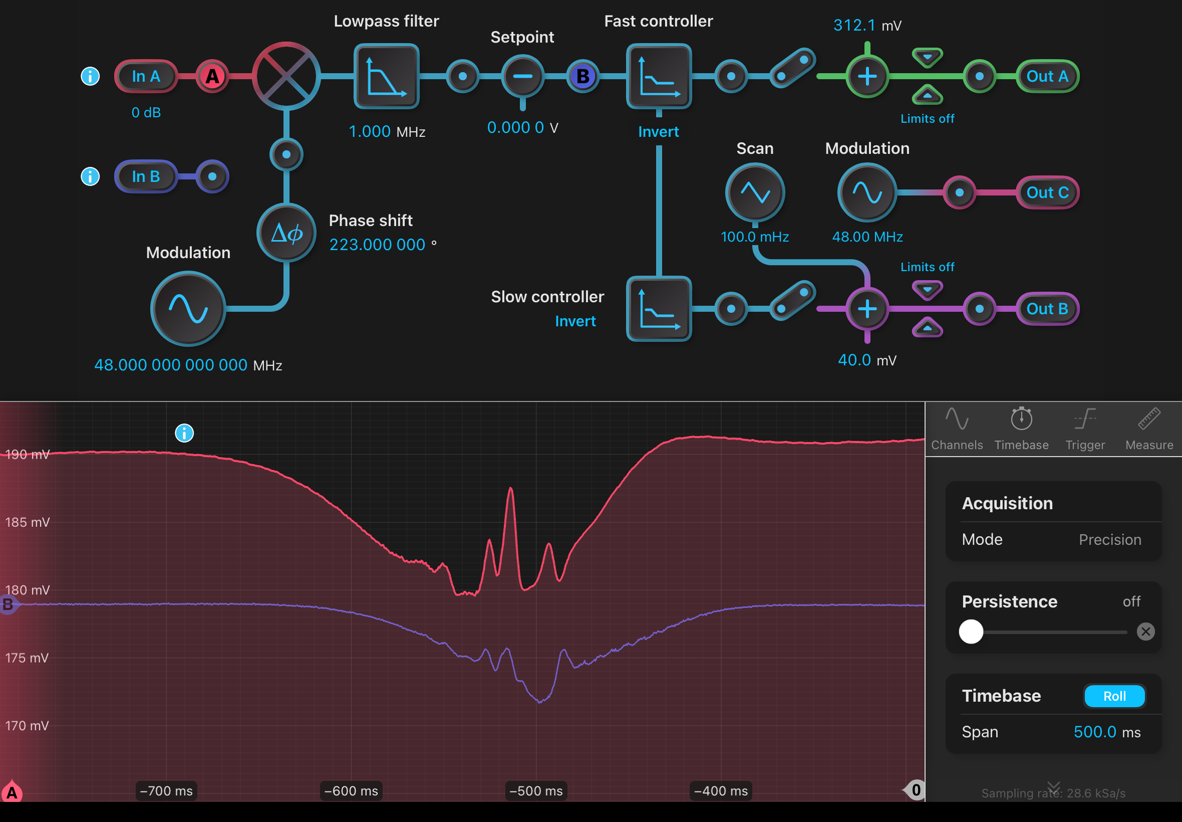
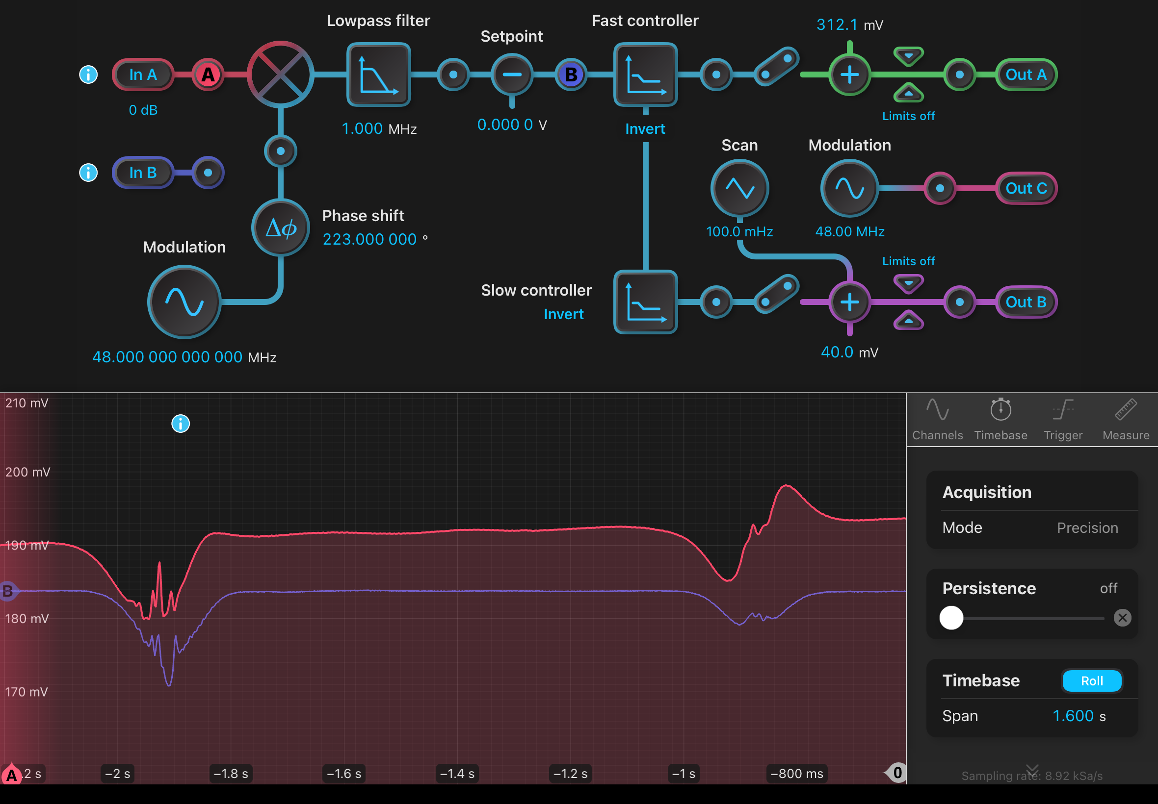
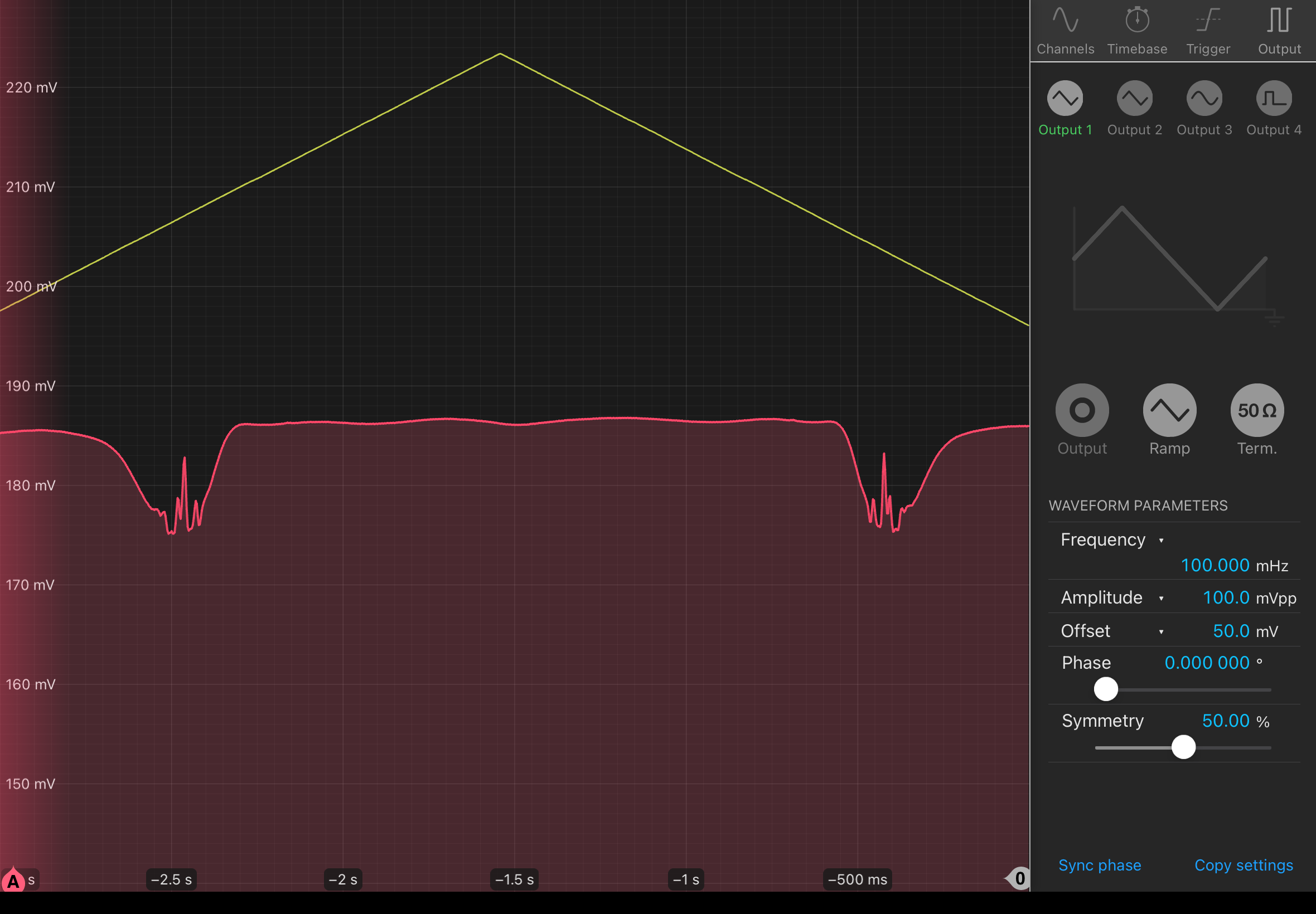
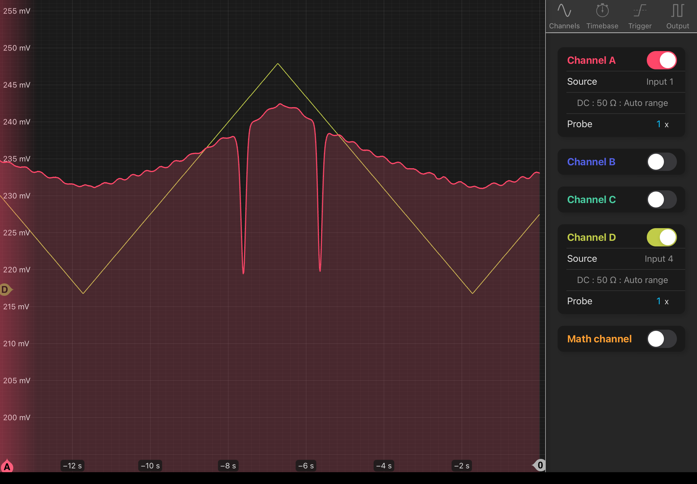
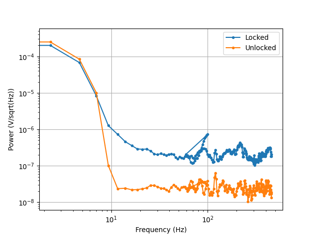
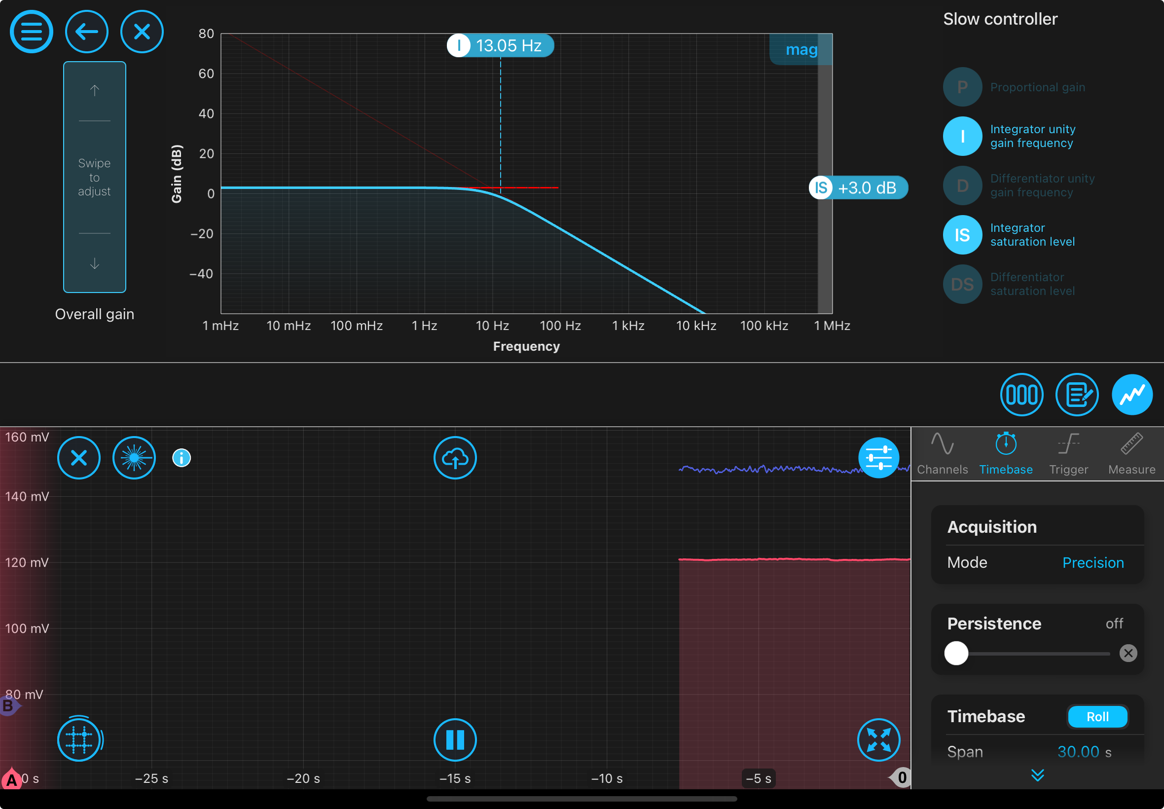
Took data of the pump, will analyze this to see what hyperfine transitions they correspond to. Pump fell out of alignment so needs realigning. On Tuesday, we achieved lock! We took 20 seconds of 5000 samples per second for the locked and unlocked cases using the same method as with the probe and we get the following PSD: pump_noise_spectrum.png. The unlocked case has higher noise than the unlocked case, which is what we would expect. It is not immediately obvious why this seems to behave as we expect and not the probe, but I wouldn't trust it yet since we did this very quickly and only once so far (also the modulation frequency/phase/alignment were not optimized). Slow controller used and error signal: controller_20240813_193716_Screenshot.png. Blue dot in image shows the peak that we locked to. Also, the standard deviation of the error signal when locked was ~2.12 e-6 V whereas when unlocked, it is 3.72 e-6 V, which also matches with what we expect since the error signal would be greater and fluctuate more for an uncontrolled unlocked laser.
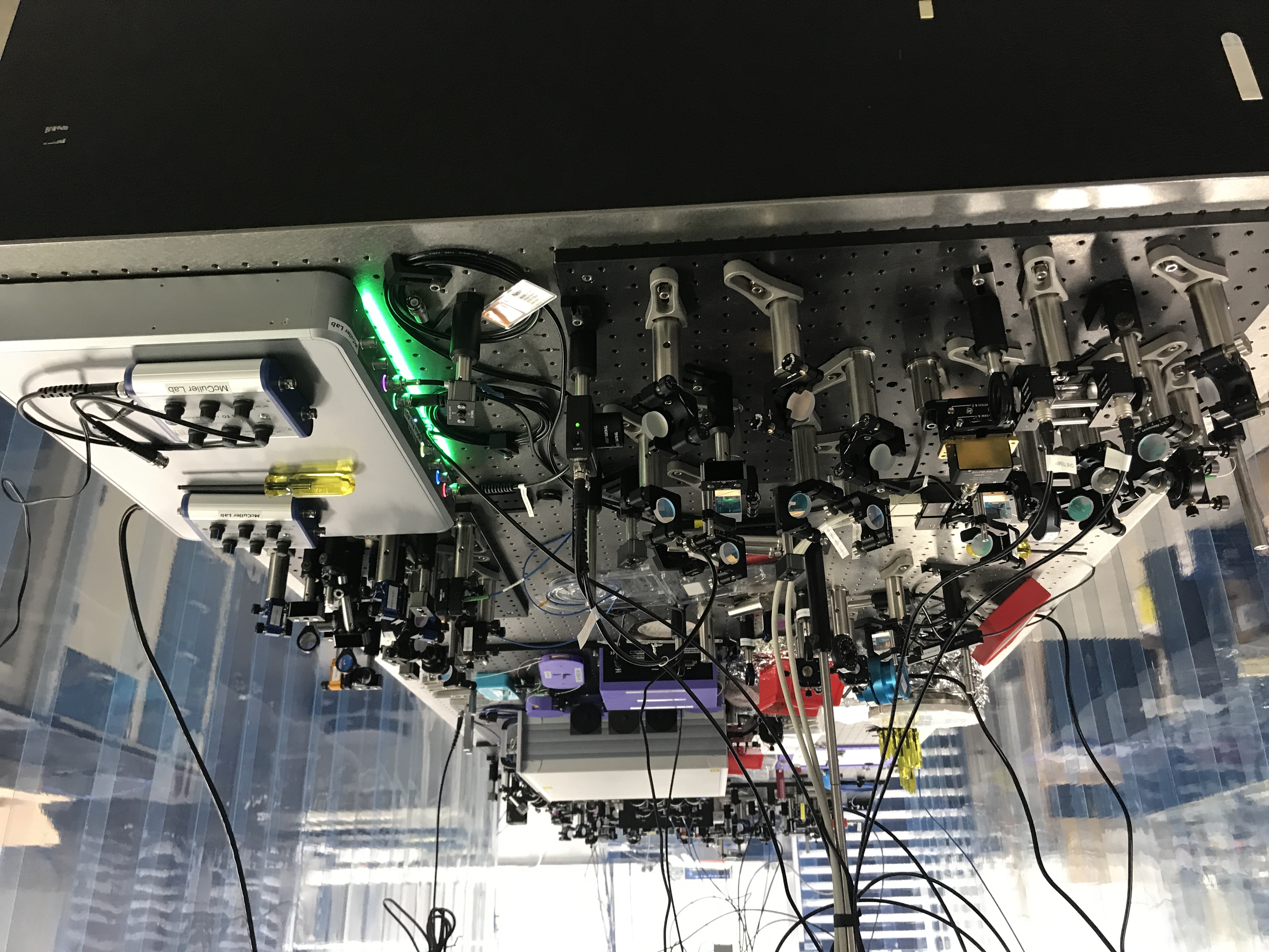
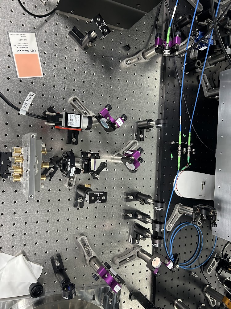
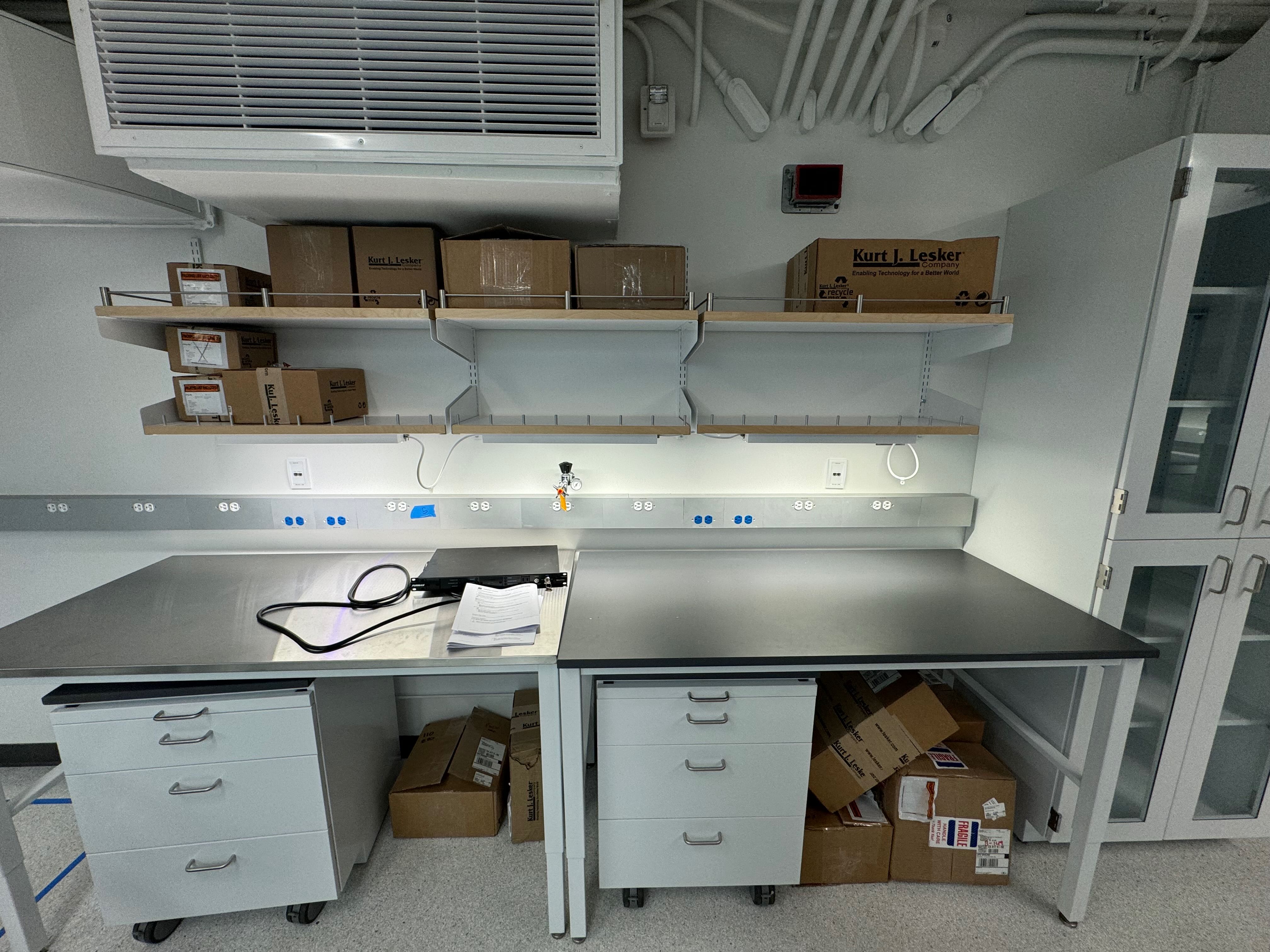
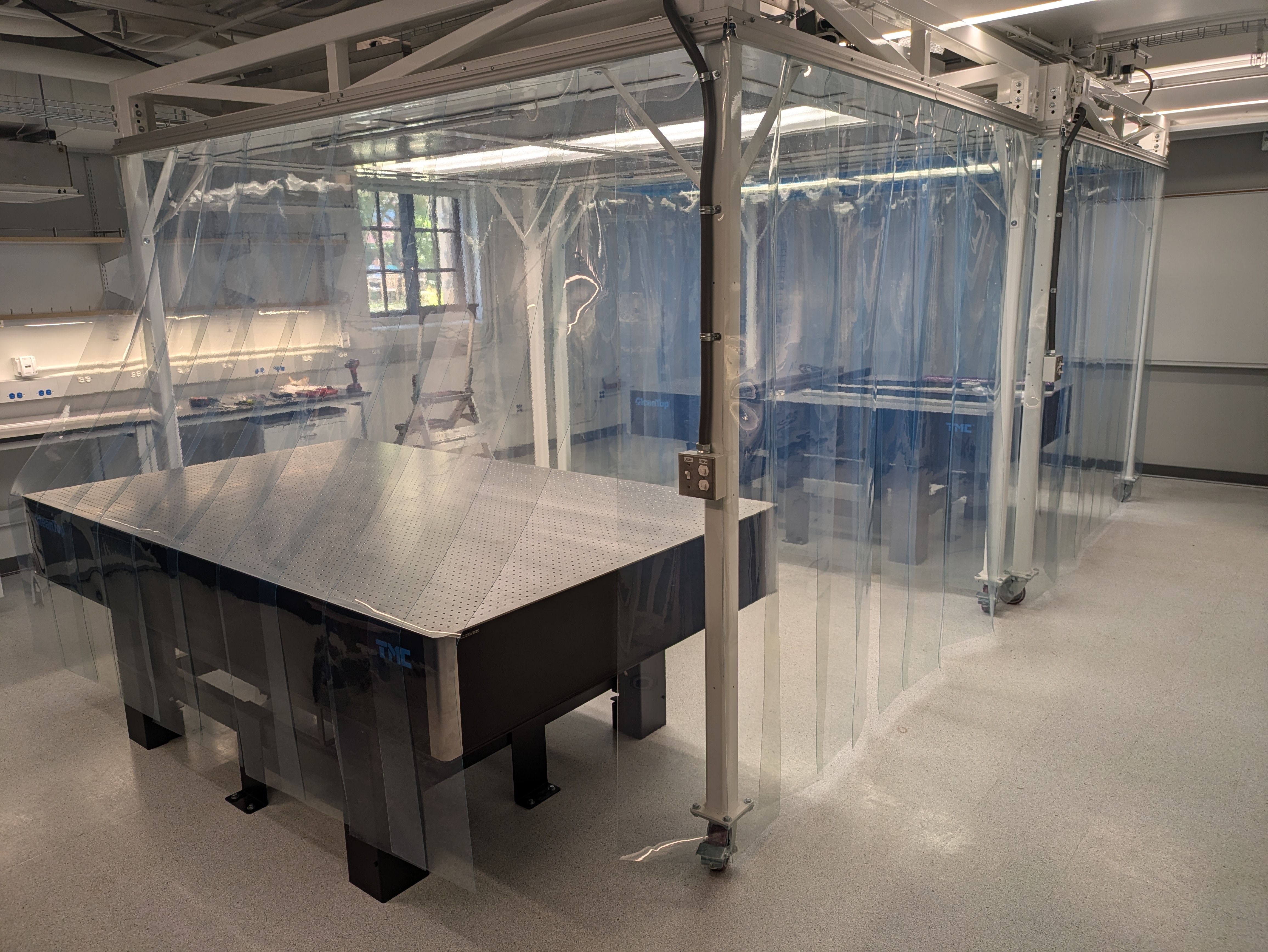
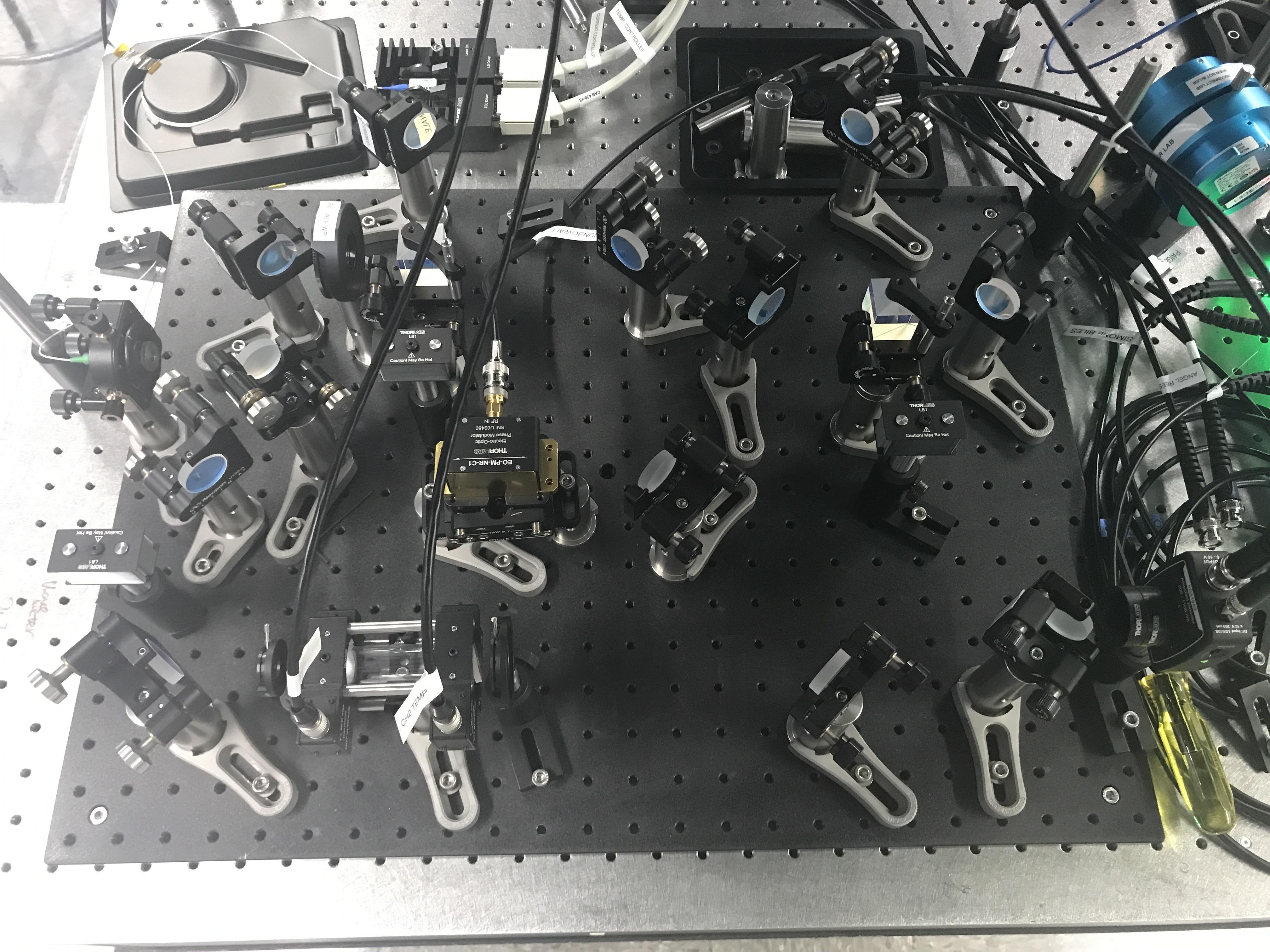
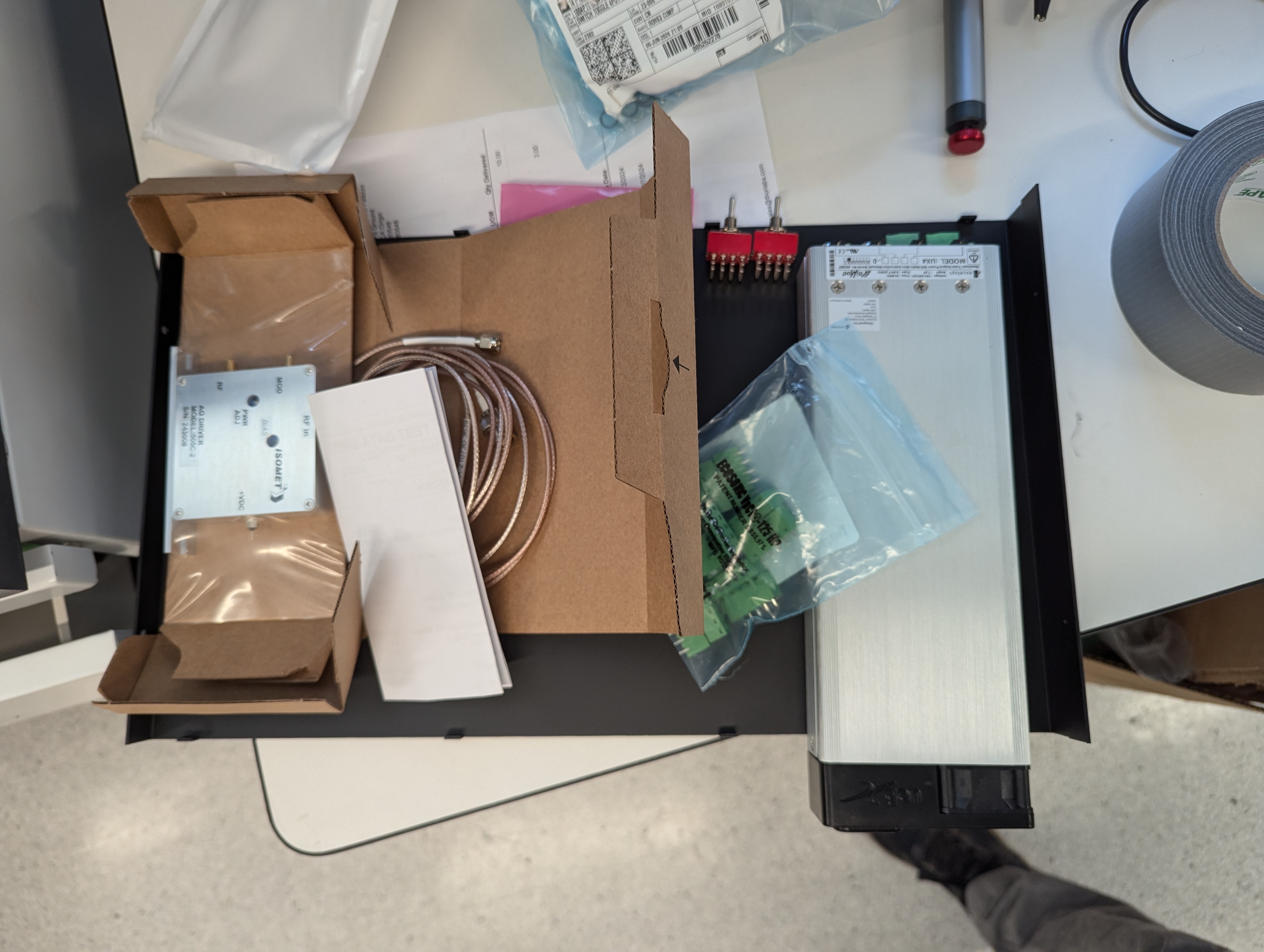
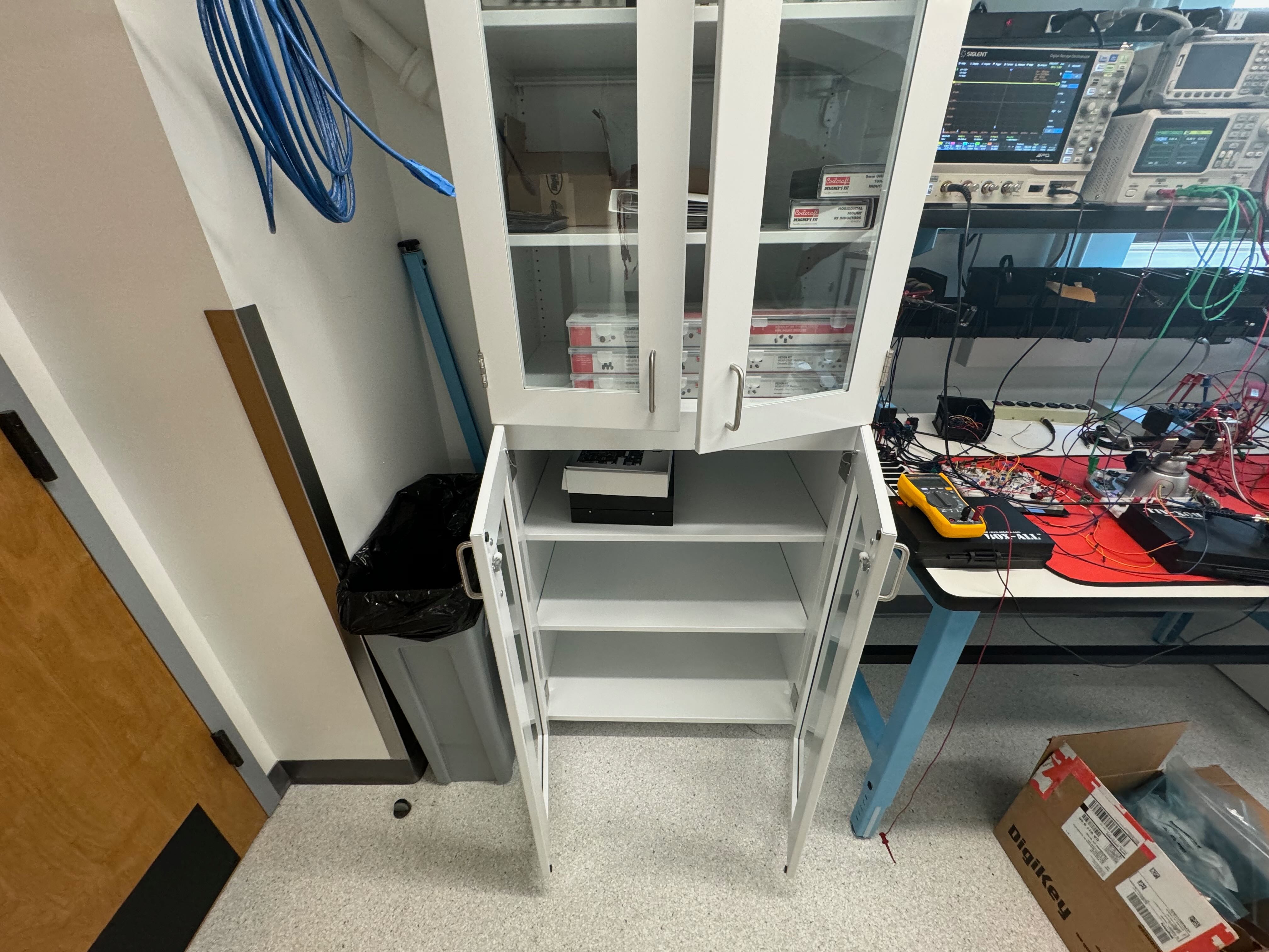
Current setup: IMG_2454.jpg