Gain Margin and Phase Margin Relation

Using the calculated \( H_\infty \) limited controllers in the attached plot I show that as \( \gamma \) decreases the phase margin and the gain margin both increase. It also shows that the gain and phase margin are strongly correlated. In the plot the gamma is represented by the colors in the color bar and the current LIGO controller is shown as a blue triangle. The different lines of points are diffrent F1 gains and show that the relation between the gain margin and the phase margin is not always linear. However, generally speaking, this shows that gain margin and phase margin can be used somewhat interchangeably in this case. I'm not sure if this extends to all admissible controllers.

Mathjax? Adding Latex to the Logbook

When \(a \ne 0\), there are two solutions to \(ax^2 + bx + c = 0\) and they are \[x = {-b \pm \sqrt{b^2-4ac} \over 2a}.\]

The source for this is:

When \(a \ne 0\), there are two solutions to \(ax^2 + bx + c = 0\) and they are \[x = {-b \pm \sqrt{b^2-4ac} \over 2a}.\]

Note that text inside of

, 

tags does not get rendered. The ASCII Text edit mode uses those tags.

 

Chris's current Shipping list

From Chris, attached pdf shows pictures of all of the vacuum pieces to review.

Packing List for Vaccum Shipment from Fermilab to McCuller Lab

I'd like to finish gathering parts for shipping and get them over to the carpenter's shop, where they will be put into shipping crates. What is the shipping address we should use? Where is the list of items you request? We have staged the following to be forklift accessible: quantity 2 central vessels; vibration isolation quantity 4 cubes Other items in the tunnel can also be moved now. Please point me to the list you are preparing of other items and quantities to ship: T-sections ion pumps gate valves edge welded bellows formed bellows short tubes (to be measured again, or does Daniel have the measurements?) all windows removed from vessels assorted blank flanges, bolts, nut-plates, and conflat flanges. valves what else?

Manipulation for Unstable Environmental Noise Model

[Continuing 11217]

The environmental noise (SEI) must be stable and the plant must have a nonzero D matrix. Because the controller I added in [11217] was unstable it made the seismic section unstable causing the failure we saw in the last post. To fix this issue I manipulated the poles and zeros in this way;

1.  Copy all unstable poles into the plant as new poles of the plant
2.  Make the real part of all the unstable poles in the SEI negative, thus stabilizing the SEI.
3.  Copy all the newly stabilized poles from the SEI and make them zeros of the plant. Make sure you are only copying the poles that were unstable before step 2 and not all the now stable poles.

This process keeps the SEI stable and keeps the plant's D matrix non-zero all while keeping the characteristics of the system. The stable poles in the SEI are canceled out by the zeros in the plant leaving only the unstable zeros in the plant. 

When running this modified model, the solver runs no problem and gives the attached RMS plot. This plot has all the features that we are looking for; the margins increase as we move away from the H2 limit and it does not seem to have any numerical errors. 

There are two things that bother me about this plot. The first is that the current controller (red center in the top left of the plot) seems to be in the outside the theoretical H2 bound for optimality, i.e. it is to the left of the dotted red line. One possible explanation is that this might be some numerical thing, for example, it is not unusual for the solver to return controllers that were below the theoretical limit when the controllers seemed to have numerical issues like the BNS FOM being weighted too high. The second of which is that the current controller does not seem to be particularly stable with this new model. It is only reporting 0.55dB of gain margin and under 10 degrees of phase margin. I'm not sure why either of these things is true and I haven't investigated yet.

There are a few things that are new with the plot. The first of which is that there is an H2 optimal bound on the plot. This is the red line. The second is that there is text to describe what the numbers next to the points are. This is ground breaking tech

Next Steps:

1.  Talk to Lee and finalize the ASC model for the paper. This involves deciding on the SEI and measurement noise levels are that make sense.
2.  Add the getSPOFF() to buzz and add the new pole/zero manipulation to it in case of unstable environmental noise.
3.  Update the solver with the slightly better solver from Lee.

SNSPD Update

I have been working with Boris in Maria Spiropulu's lab to learn and develop some of the ground work to characterizing and achieving the dark noise levels needed on the SNSPD's for GQUEST. Thus far, I have been working on the development of a new base of python libraries for interfacing with the new frame controllers packed with a laser, attenuators, switches, and a power meter, all used for taking measurements of laser power amplitudes and characterizing the SNSPD's. Today I have finalized the code library for controlling the Yokogawa AQ2212 frame controller as well as the GRID TLS Laser Module, attenuator modules, OSW switch module, and power sensor module over ethernet. This library has been compiled in python and I have successfully completed testing on my overall control of the system today. The tests I have run so far have been to first completely setup all appropriate parameters (via the python commands over ethernet) such as: laser wavelength (1550 nm), laser power (10mW), attenuator attenuation (30dB), attenuator wavelength (1550nm), switch routing (between on board power meter and a separate Thorlabs PM100D, and finally reading the power meter in single bursts or continuously. There also exists controls for turning on and off the laser output and each individual attenuator output. The test initiated all of these subsystems successfully, took 10 data points from the power meter and averaged them, swapped the output to the Thorlabs power meter, then turned the system off and disconnected from the device without issue. The results can be seen in the attached images. Average power (on board) 6.02 pW, Thorlabs reading average 6.04 pW The next steps will be to carry over this code in an implementation of Andrew Mullers code to perform characterization tests on the SNSPD's. I will follow his workflow for performing the experiment, and we will then carry out a test using my updated code for the new equipment and compare it to a new test using the previous code and older equipment. This will be done sometime next week. Lastly, I will be creating a gitlab project to store all code I develop and manuals necessary for understanding and performing the experiments we do on the SNSPD's. image 1 - current setup image 2 - readings from the yokogawa frame controller during test image 3 - readings from the thorlabs power meter during test image 4: It should also be noted, that the Laser trigger control must be shorted for the Yokogawa frame controller to allow the unlocking of the laser output control

PCB Update

For ordering electronics I have spoken with Dean and he has suggested the following: Screaming circuits is a good place for stuffing the boards and he uses them frequently without much issue. As for the PCB fabricating, he suggests that we use Sunstone: https://www.sunstone.com/ Dean also mentioned that sunstone has the ability stuff the circuits via screaming circuits, so this will likely be the best option for ordering stuffed PCB's. I will be gathering the BOM and schematics needed, outlined by both sunstone and screaming circuits, to prepare possible orders for the following: https://dcc.ligo.org/LIGO-D1300671 (Homodyne Detector) https://dcc.ligo.org/LIGO-D2000388 (MIT DC QPD Circuits) And the whitening board that I will be further modifying using the Max333A logic switches (TBD). I am waiting on the MAX333A chips to arrive to do some final testing on before finalizing the schematics. (refer to servo components schematic... https://awiki.ligo-wa.caltech.edu/wiki/LabAmp) https://dcc.ligo.org/LIGO-D1001530 (aLIGO ISC Whitening Board) Lastly, Dean had no real preference on BNC cable brands for making our own, he suggests we just purchase pre-made BNC cables.

Options for IR Laser Viewing Cards

[Ian, Torrey]

There are a few options for good viewing cards for 1550 nm. I lay out some of the options here. A good resource is this Adakari Group elog post 

1. ThorLabs VRC2 ($94) is a good option and is made of durable plastic. They are currently used in the Cryo Lab but the VRC4 may be better. Might be hard to punch holes in. Both ThorLabs cards have the same minimum detectable power which seems to be comparable to or better than the Newport F-IRC4. 
2. ThorLabs VRC4 ($94) Same build as the VRC2 but sensitive to narrower bands (790-840 nm, 870-1070 nm, and 1500-1590 nm).
3. Edmund Optics Laser Detection Card This used to be cheaper but may be good to test. I haven't used it before.
4. Newport F-IRC2 ($195) This is the card I see most often it has a minimum detectable power of 8 µW/cm²  from 800-1700 nm and is laminated so it would need to have holes cut carefully. It also comes in smaller and cheaper sizes (See F-IRC2-F, and F-IRC2-S). This is also used in the Cryo Lab.
5. Newport F-IRC4 ($205) Basically the same as the Newport F-IRC2 but with shifted bandwidth (700-1600 nm) and lower detectable power (3 µW/cm²).  Also comes in one smaller size (See F-IRC4-S)

We should get a variety for different applications and also to test them out. we will spend a lot of time looking at them so we really do want them to be good.

Set Up Temporary Soldering Station

[Ian, Torrey]

We set up a temporary soldering station in the swing space. this is just until the full lab ins built then we can move it over there. It is also so that we could move all of the electronics equipment off of the optical table. it is very crowded right now so we should buy some storage for all of the stuff to clean up the area a little bit, but for now at least it is off the optics table. We also need to order some solder because we don't have any.

See picture

Added Network to Swing Space

I set up the network for in the swing space. Both the 2.4GHz and 5GHz networks combined into one network. We can turn off the 2.4GHz network if it starts to be a problem. 

Router model: ASUS - AX6000 Dual Band Wi-Fi 6 Router, Model: RT-AX88U Pro

Network Name: pLANk time

Network and Admin Passwords: LIGO Secrets or written on router

Admin site:  http://192.168.50.1

cryo lab update and unknown oscillations request

The Mach–Zehnder in the cryo lab was installed with a beamsplitter mounted on a 3 port mount. Went to install the second readout of the Mach–Zehnder and discovered this. I have since reinstalled the beamsplitter with an appropriate mount, put the other 1811 PD with a lens in front of it on the second readout path, and recovered the alignment on both paths. Minor alignment is still needed to maximize visibility but there are fringes.

 

Additionally, the source of the oscillations on the PD in reflection of the cavity are still unresolved. Here are some things I know about it:

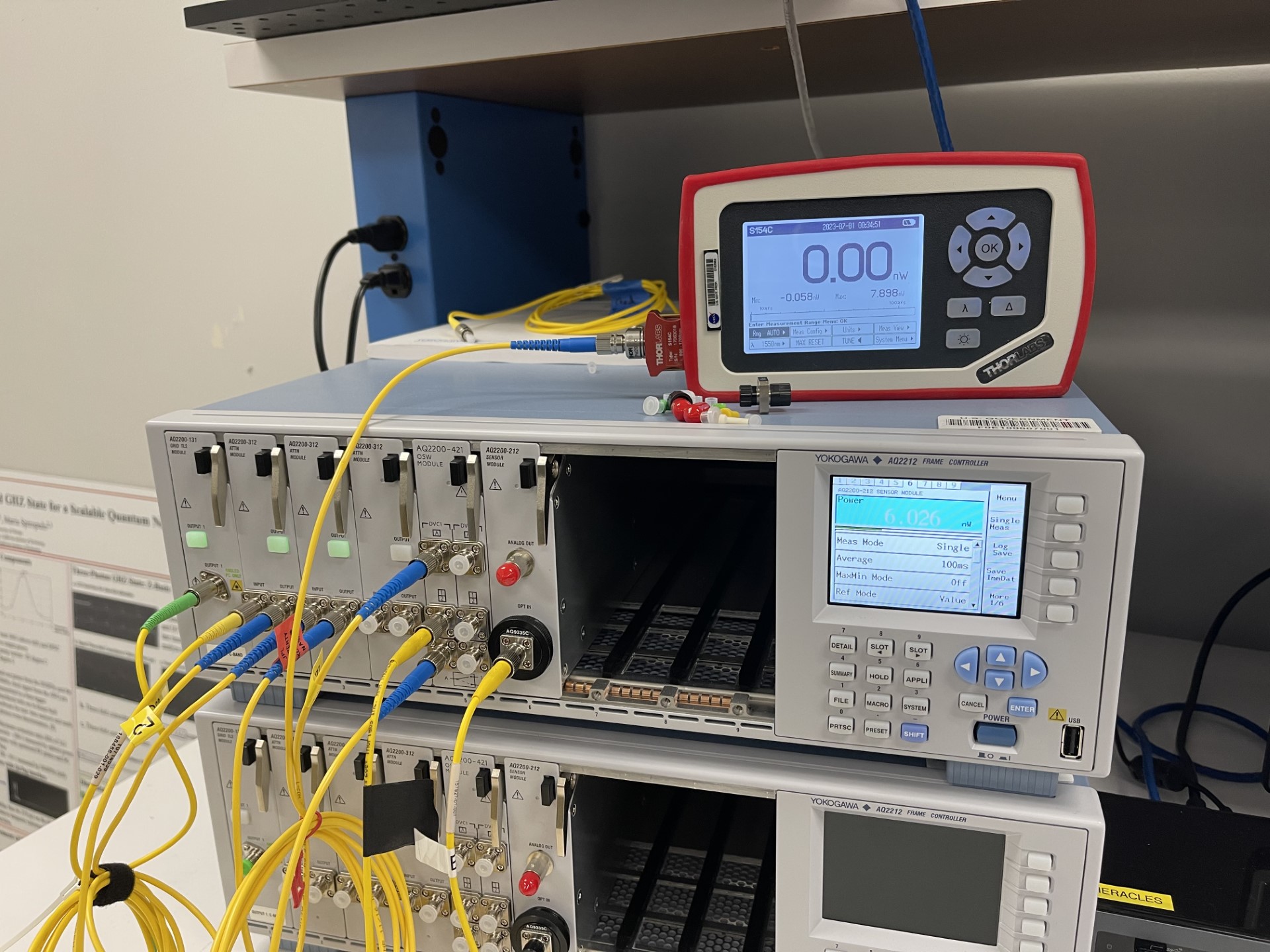
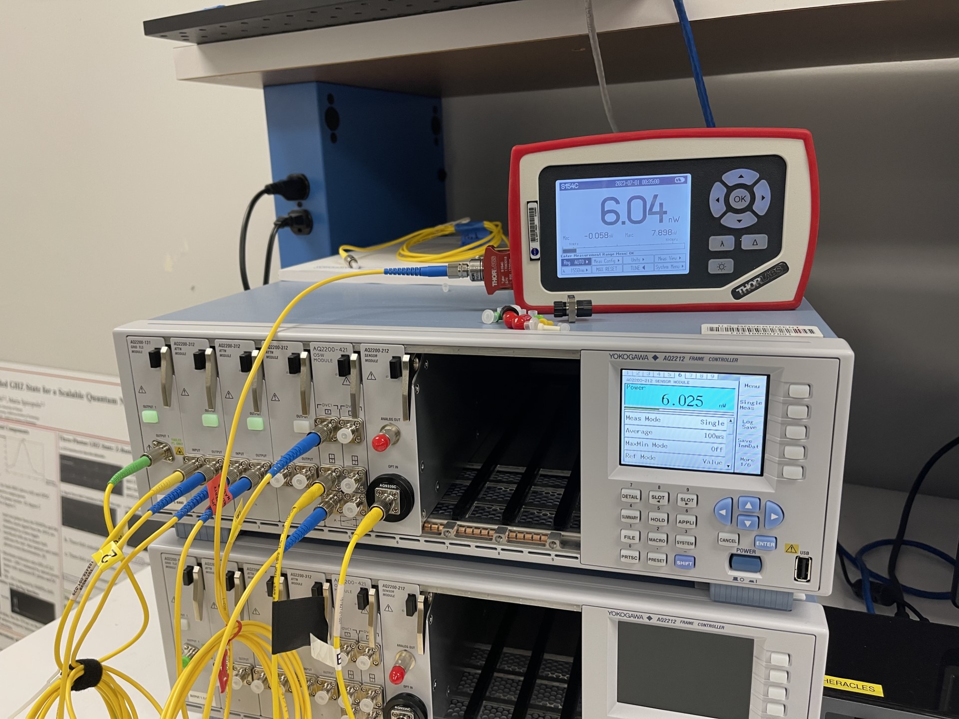
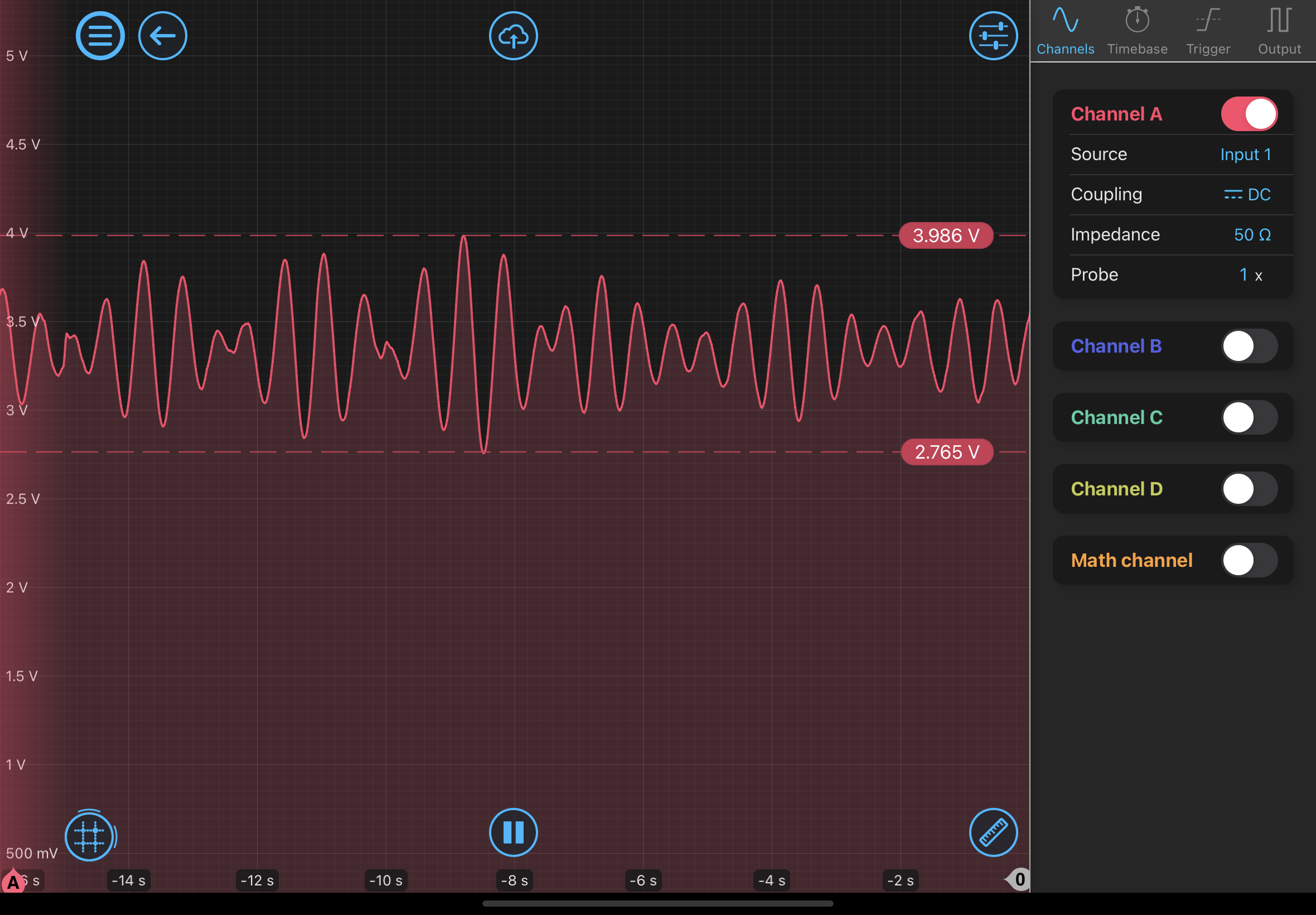
1) I don't believe they are physical power fluctuations with the laser. As you can see from the screen shot, those fluctuations are between ~3-4 volts on the PD. If these were physical power fluctuations they would show up on a power meter; they don't.

2) They don't seem to be a saturation issue as you can use the half wave plate + PBS to control the amount of power to the cavity and they still occur at very low power.

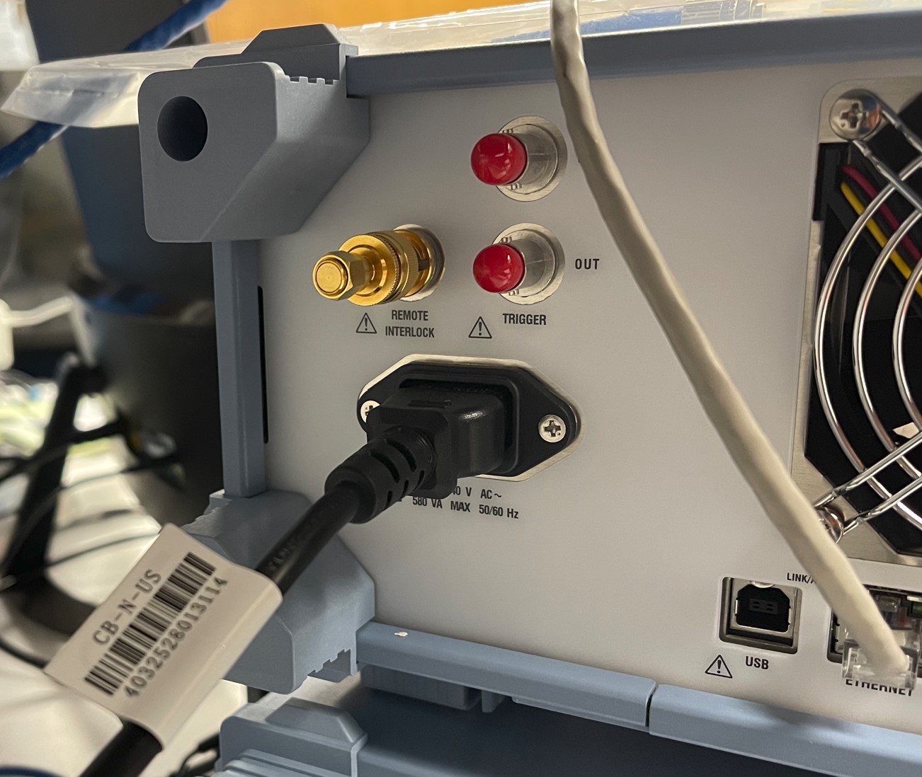
3) Thought maybe an electrical issue. I substituted the power source for a new 15V power source that we just bought from Newport. Aaron suggested having the moku and PD power from the same power strip so they have a common ground. Also I've tried plugging in the PD to different outlets all around the room. Nothing has worked.

4) The new 1811 I installed in the Mach-Zehnder path (that doesn't see the cavity at all) does not have these fluctuations.

My only other idea is maybe the suspension of this chamber that the cavity is housed in (if it has a suspension) is causing it but I'm unsure how to mitigate/test for that. If anyone has any ideas, please let me know.

Using non-stabalized ASC model in Buzz

In all previous tests I have been using a model of the ASC system that was fit from data using IIRRational in the 'ASC' Folder of the 300m repo. The ZPK representation (See attachment T_ASC_CHARD_P_Unstable.yml) that it produced had right half plane poles meaning the filter was unstable. We then stabilized this by hand by flipping the right hand plane poles into left hand plane poles, i.e. 4.9234+12442i  -> -4.9234+12442i (See attachment T_ASC_CHARD_P.yml). We then used the stabilized version in all of our testing. 

I went back and tried to see if the solver could handle the the unstable ASC model. I added the model  (See attachment ASC_BH2_solver2_unstable.mat) to the buzz 'ExampleModels' folder in the buzz repo and tried it. The solver fails when calculating:

'Q = solve_continuous_are_scipy(a=A.T, b=C.T, q=V1i, r=bh.D2 @ bh.D2.T, e=None, s=V12i, balanced=True)'

giving the error:

'LinAlgError: Failed to find a finite solution.'