I successfully locked the cryo west cavity using the laser lock box on the moku yesterday. The main catalyst to this was that the PD being used to measure the REFL signal had a bandwidth of ~10 MHz and was attenuating the 32.7 MHz modulation signal. We ordered some newport 1811 PDs (BW = 125 MHz), and the modulation signal shot up by several orders of magnitude. Note that there is now a lens in front of the REFL PD because the diode on the 1811 is very small, also the damage threshold on these is MUCH LOWER than some of the thorlab equivalents. Don't send > 1mW towards the cavity.
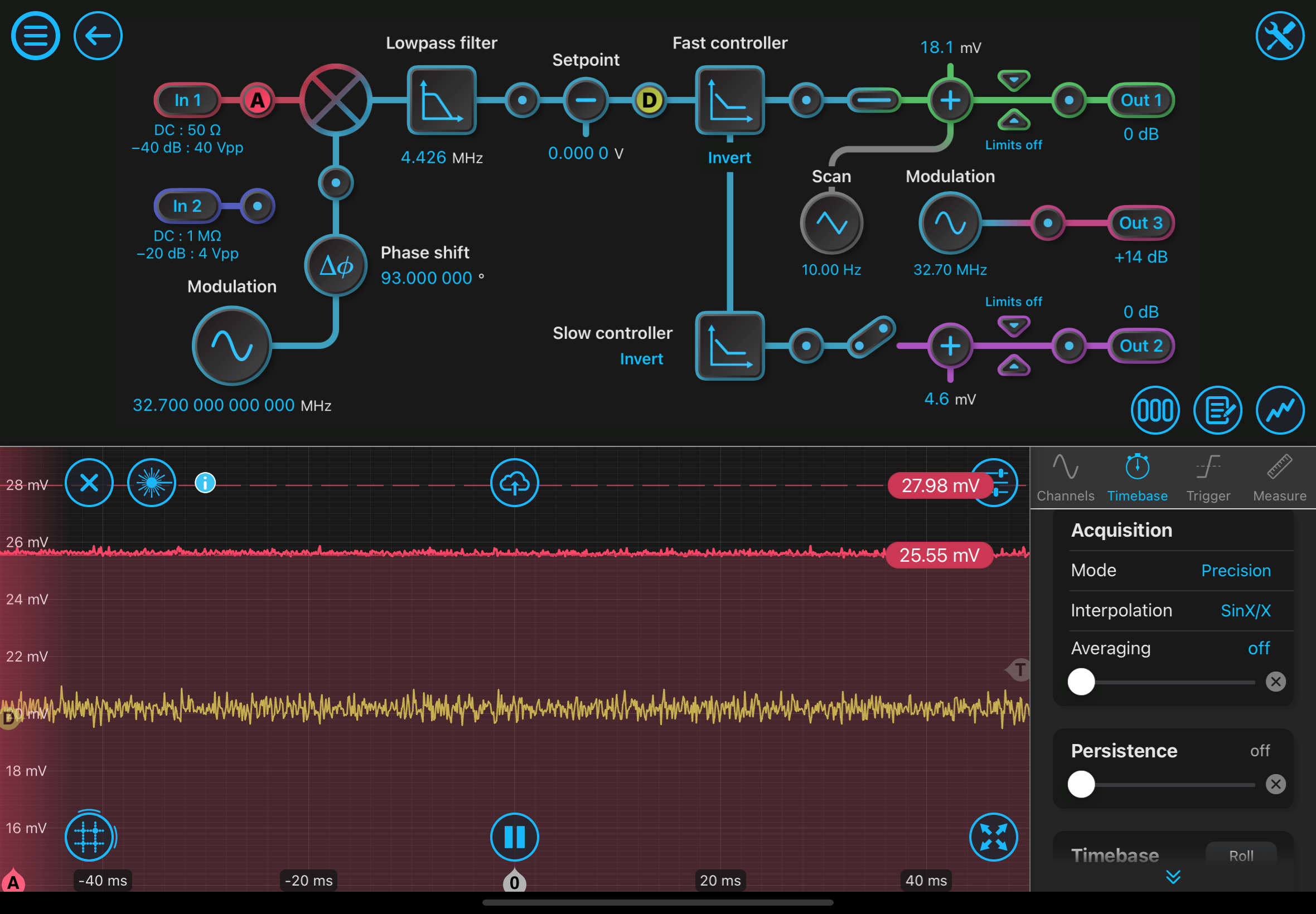
First, the settings of the laser lock box that were used for initial lock can be seen in the attached text file, as well as a screen shot of the lockbox while locked. The process I was using was:
1) Make sure the TEC setpoint is roughly centered to ensure maximum range on the slow loop. Manual engage the slow loop.
2) Slide the slow loop offset until its roughly near the cavity resonance, i.e. you see the large dip in REFL PD.
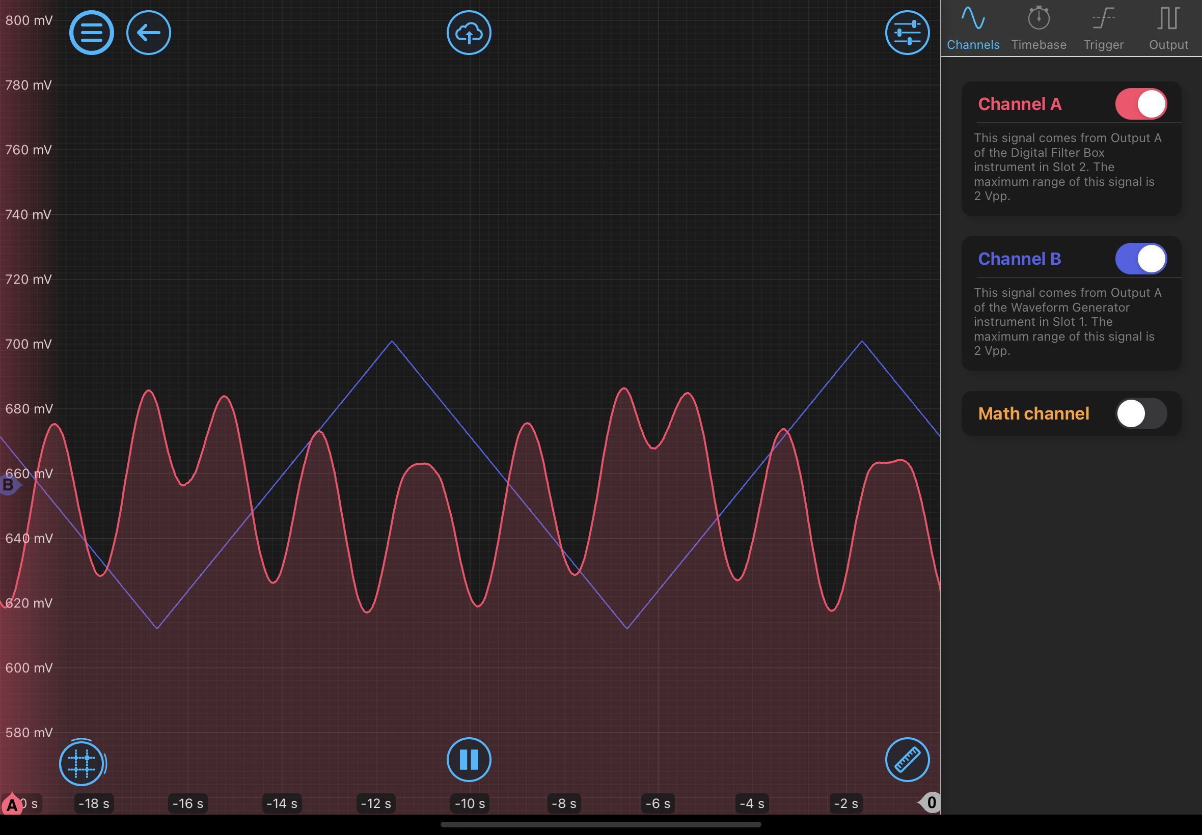
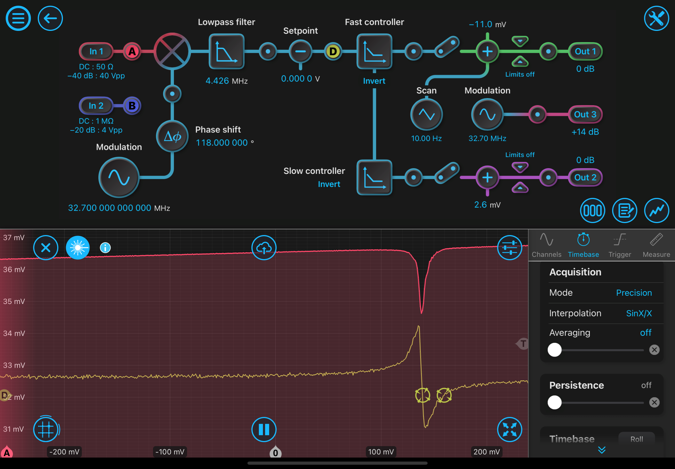
3) Engage the laser lock box assist function, which is this button. You should now see the REFL PD dip is centered on the error signal zero crossing point, along with some cross-hairs highlighting the zero crossing point on the error signal. These are clickable. Click the zero point that corresponds to the RELF PD dip (sometimes the moku adds additional cross-hairs that are garbage). I'm realizing I don't have a screenshot of this, I'll grab one and comment on this post with it later today.
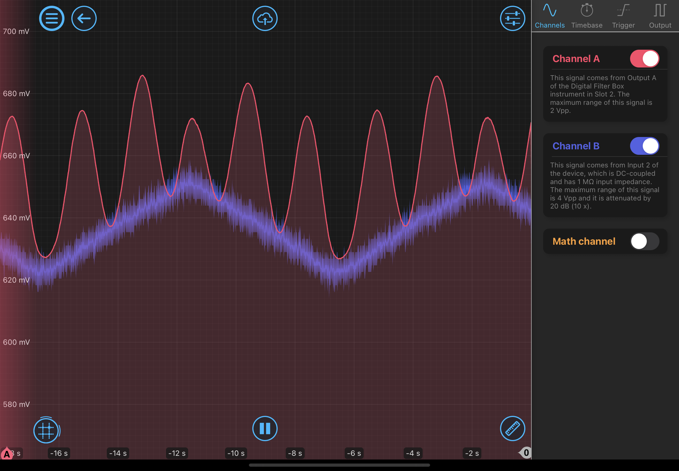
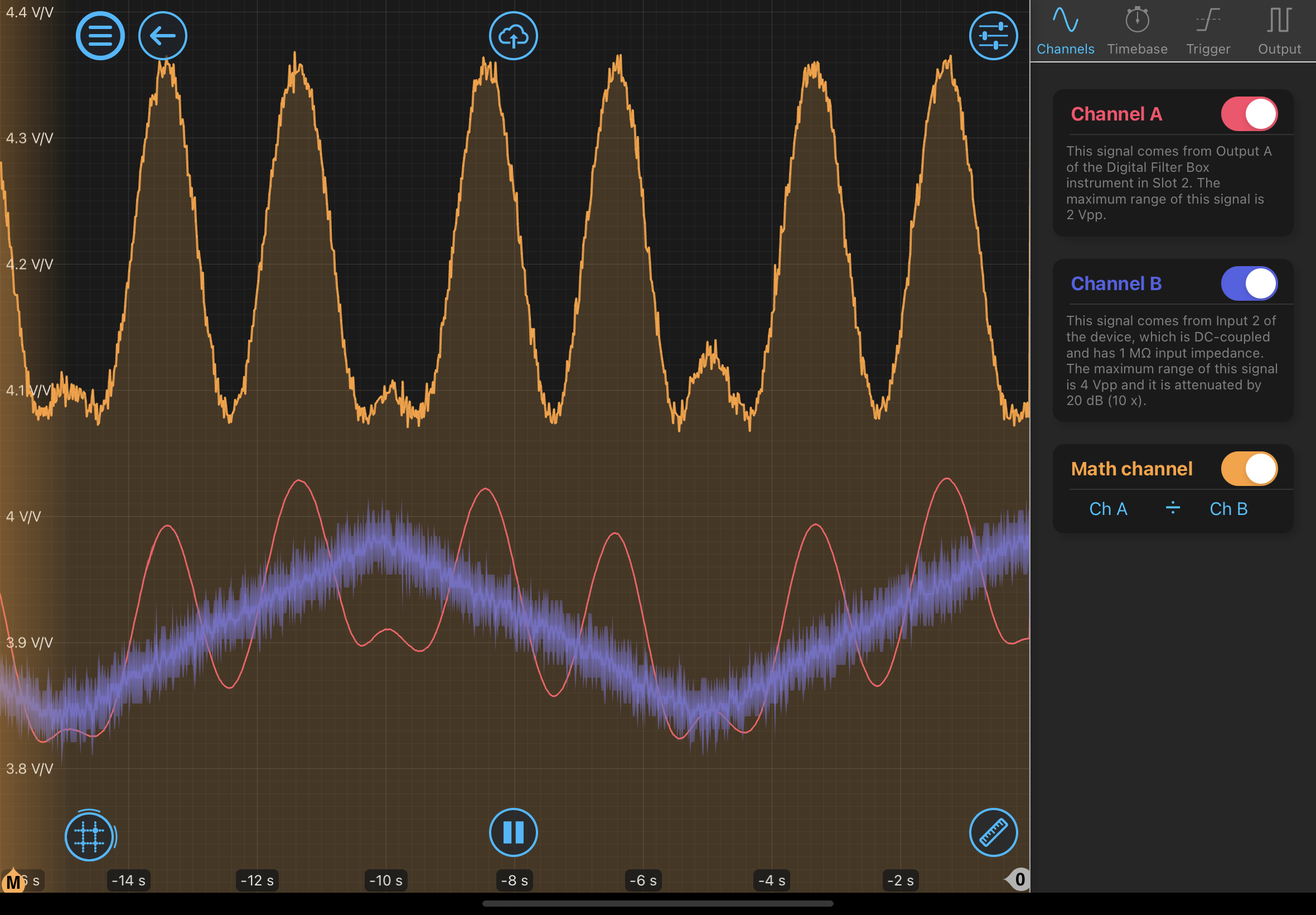
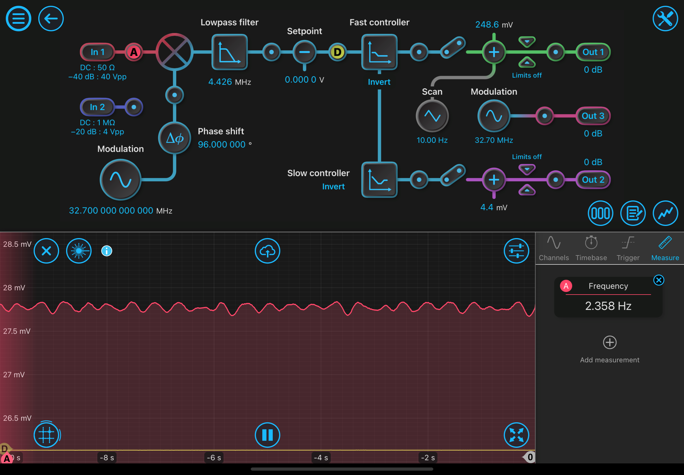
And thats it! Pretty easy with the moku once everything is set up. I kept the cavity locked for 10+ minutes while tapping the table, the lock seems fairly robust. A minor nuisance, in the other attached photo there seems to be some random low frequency oscillations on the REFL PD that I'm unsure where its coming from.
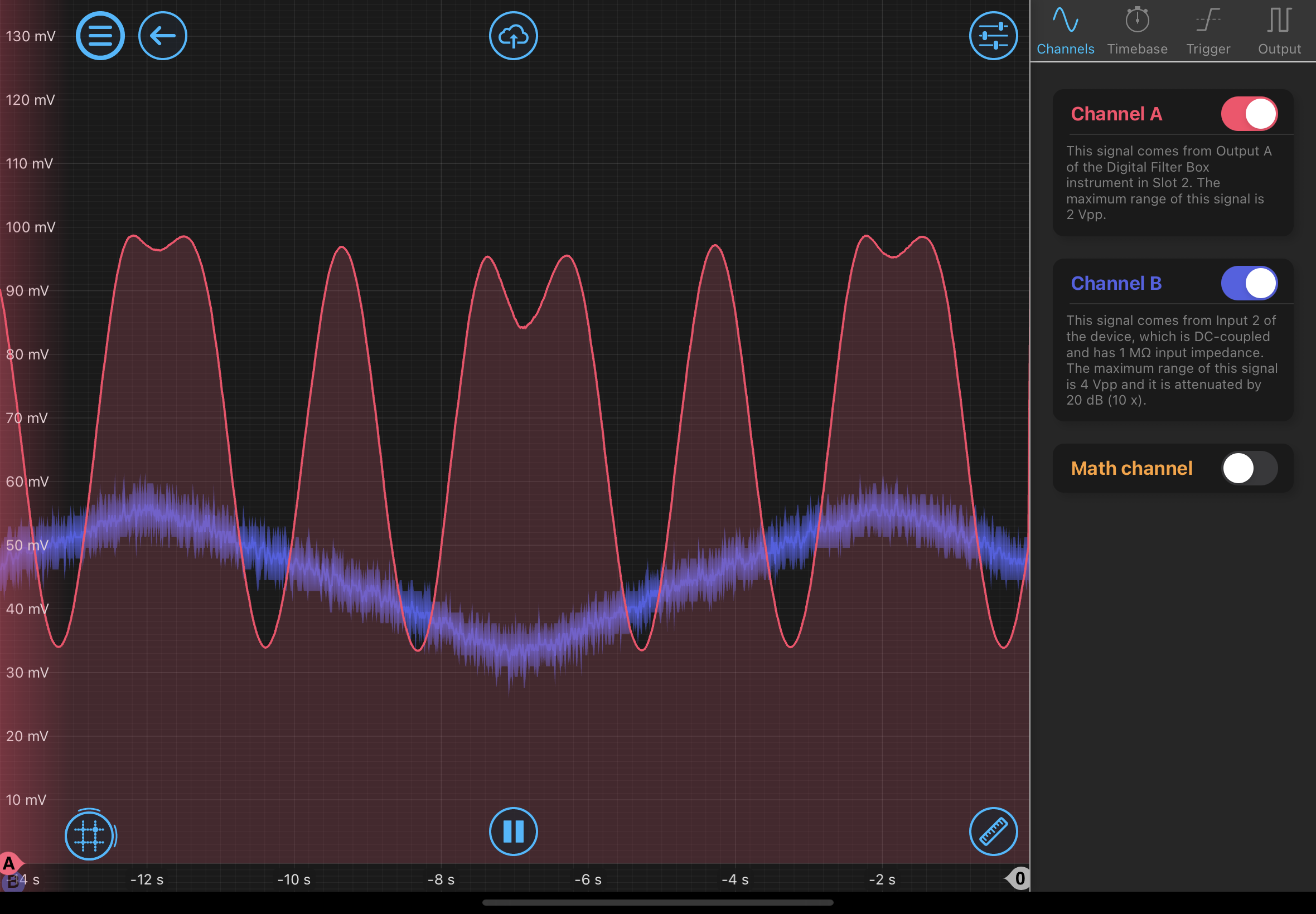
Example of zero point crossing when using the lock assist function.
Laser's steady hum,
Cryo cavity now locked,
Early victory.
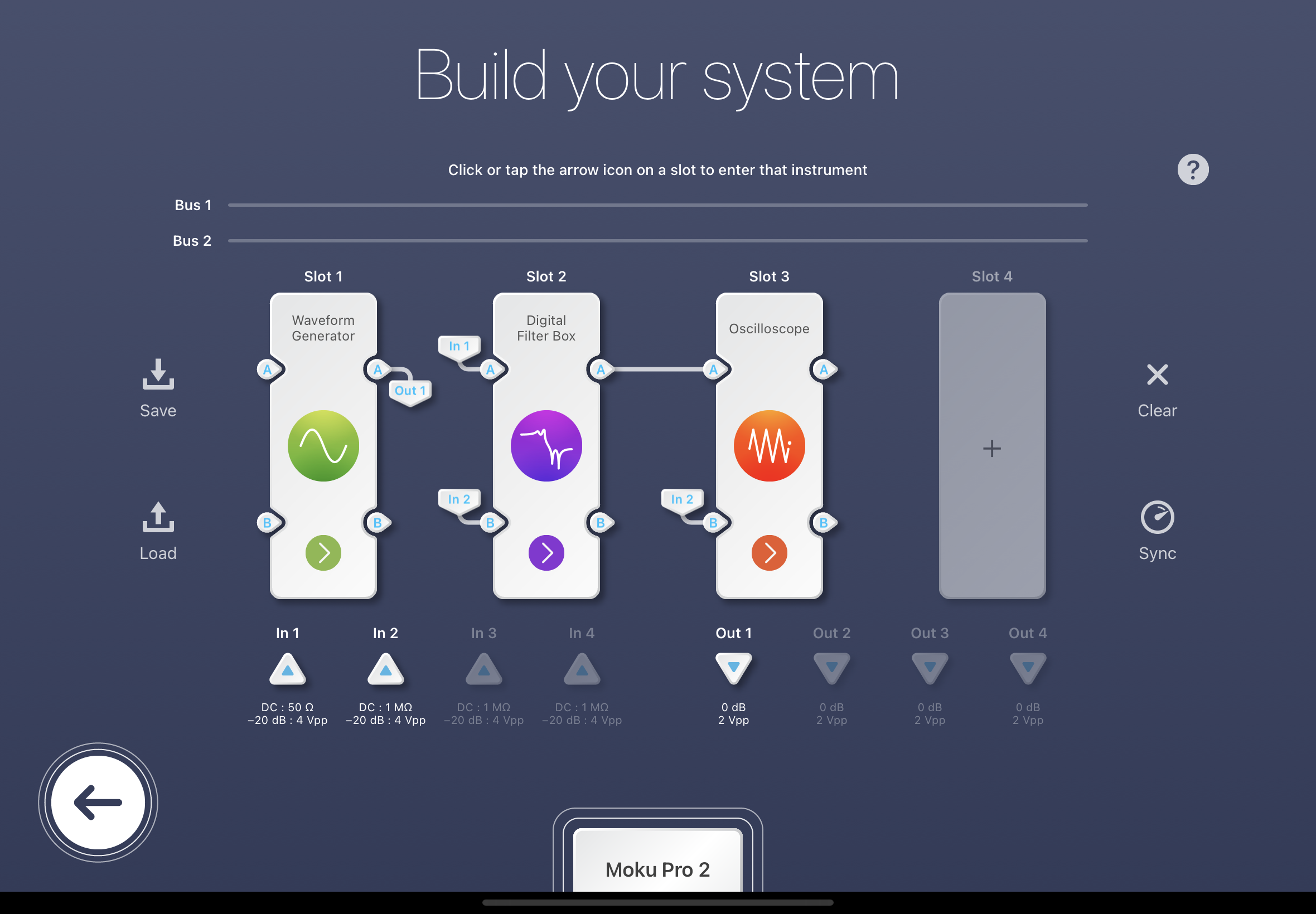
Diagram of current setup when lock was achieved.
I tried the LSC model (tried attaching but does not accept .mat files) with the H2 solver And it worked like normally. You can see these results in the "LSC_H2_Results.pdf" attachment.
When trying the LSC model with the H2/Hinf Mixed solver it struggled to recover even the H2 results. This is with a gamma going from 1e3 down to 1e-1 (not igsq). On the H2 result it looks like the Closed loop is peaking at about 100 so this should be plenty to at least recover the H2 results. but I am left with the results seen in "LSC_H2HinfMix_Results.pdf"
It is possible that this is a problem with the Zinf connection but I will have to investigate further. I also still need to try the damping loop. Also I got multiple color bars working using This.
I am running into a problem choosing the color scheme for the plots for the paper. There are two main challenges to this first is that in the mixed H2/Hinf case the color conveys two pieces of info: the FOM weighting and the gamma limit on the Hinf norm. I have attached a number of single color schemes in the "PaperALS_OL_BODE_colors_comp.pdf" attachment. I don't know how to handle the gamma limit. Ideally there would be a 2d color space to map like in the pycolormap-2d package. Is it worth it?
The other main plot is the RMS plot which also has two color schemes one for the gain margin and one for the FOM weighting. This is easier as long as the colors don't overlap. Also I haven't gotten the dual color bar to work on the RMS Plot. the scaling always is removed by adding the second color bar. See the example RMS plot in "PaperALS_FOM_RMS_Scatter.pdf"
Note: some of the colorbars are messed up in "PaperALS_OL_BODE_colors_comp.pdf"
Remeasured the frequency noise with the 785 after the visibility improvement. Assuming my calibration to Hz/sqrt(hz) is correct, the measurement is still yielding several orders of magnitude larger than what rio claims it to be. Investigating this today.
For reference, the SR785 measures a quantity is V/sqrt(Hz). To convert to frequency noise I do S / (L/c * B*2*pi) where S is the measurement, L is the path length difference between the two arms and B is the fringe amplitude. V/sqrt(Hz) / (m/(m/s) * V) = Hz/sqrt(Hz).
The right axis (Hz) on this plot has a different frequency dependence than the left axis (Rad). So be careful with the specification data. I agree otherwise that there seems to be an excess. It might be intensity noise that needs to be canceled.
Lee came into the lab today and discovered that the TEC controller's range on the integrator is very small, which is why I was having trouble driving the laser frequency. If you center on this range (~10.2 kOhm) you can then drive a signal into the back of the TEC so that there are constant fringes on the Mach-Zehnder read out. I did this via the moku (15 mV @ .1 Hz, corresponds to roughly 1 fringe). "2.png" is this first attempt, red is the readout PD, blue is the driving signal. "3.png" is then hooking up a PD farther upstream to use as a power reference instead of the driving signal (see also cryolab_frequency_noise_measurement_pdf.pdf, the lighter color laser path in that is used). "4.png" is then using the moku's math channels to do (readout PD)/(power reference) to give the fringes at a constant offset. At this point its very easy to align to maximize these fringes. "7.png" shows the improved visibility. "5.png" shows the moku set up used. There are some shenanigans with the input ranges when using an oscilloscope in multi-instrument mode where you either have it on 400mV setting and its saturated, or its on 4V setting and it auto attenuates the signal by 20dB. So the digital filter box is undoing that 20dB attenuation. For unequal powers, I believe the formula is V =(2*sqrt(34*99)/(99+34))=87%, so not perfect but a vast improvement.
I drag and drop the link at the bottom of the post during editing and it should put it inline in the text. - looks like you have to be in the ckeditor for that to work well.