I have placed the new computer on one of the tables on the east wall of B111B. I cloned the disk of the NUC in B102 onto an external hard drive using clonezilla, but was unable to copy this onto the new machine becasue the NUC drive is 1TB and the new machine's drive is 500GB. A clone may still be possible using a partition strategy, but I also expect that Lee's plan to use virtual machines will make this a moot point. As of now the new machine is running windows and I have installed no additional software.

I designed some parts to secure the 1550 nm Amplifier to the breadboard. The amplifier has some slots made for a 2U 19" Electronics Rack, so I used these to attach to the parts I made.

I decided to try to use the water jet since tolerance was not too important, the parts I designed were the same thickness, and slots are annoying to make in the mill. This worked very well. The 1/4-20 pilot holes were a bit oversized (0.209" instead of 0.201" diamter) but this is well within spec. I had to tap the parts myself and then drill another hole on the mill.

See attached files and photos.

Our plan to have the laser amplifier above the optics tables on breadboards seemed like a safety risk. As seen here or here, the output connection to the amplifier is at risk of snagging on something. Since we expect watts of power coming out of this amplifier, we need to make sure we can't accident smack this fiber and cause it to come loose. I've made a first draft of a solution for this. Half inch post system and using zip ties to secure the fiber to the rigid metal. See this or this. Note that the shelf above the optics tables was moved about a foot forward to accommodate this. 

Daniel is working on a solution to secure the breadboard to the shelf.

[Ian, Daniel, Jeff, Torrey]

Moving of the optics sleds has been completed without any hiccups. Particle count pre moving was 0/0/0 and 20 minutes after things have settled 0/0/0. The mylar is still over the cavities, we will unwrap when we plan on turning on lasers. Pictures attached.

Please note that the fans in the mobil cleans rooms in B111 should never be turned off now.

Simulations in vhdlSandbox/biquad/TDF2_llcooly,ipynb plot the values of register values for the transformed direct form II difference equations and confirm that the registers S10 and S20 need not more bits thatn the input/output values.  As a function of the critical frequency of a low pass filter (sampling frequency 10 MHz) is flat.  A 16-bit integer is 15 integer bits plus one sign bit is "nbits.png"

Using then 15 bits in the fractional part gives good noise performance when fLo=1E4, but that degrades for lower values of fLo.  Here in psd.png the x-axis is frequency/fLo for different 

I've equiped Sander with a Red Pitaya to take back to California; it contains a working biquad filter bank running at 16 bits and 125MHz, using Direct Form 1 with the Scattered Look-Ahead technique. I'll continue to tease performance out of the other implementations, specifically DF2T and BQF for higher bit counts, and I'll provide firmware updates when possible. Hopefully the current version will at least allow you to get some latency baselines. The board runs Pynq so installing the newer versions should be a breeze.

The Red Pitaya is set to use a single channel, and you can program via Pynq how many filters in series you would like to put in the signal path, up to 6. Each one can be programmed independently, so in this way you can run an arbitrary filter designed with SOS stages. Do keep in mind the current limitation of 16 bits, however. Also, I didn't include a gain stage so this is probably an obvious addition to the next version.

I've set up a Github organization with all of my work on this thus far. It's set to private so if anyone wants to take a look please comment your emails in the comments. Chris told me there was a Gitlab instance so maybe I can migrate this there eventually.

I spent some time figuring out how to get the HAAS VF-2 CNC Machine to make high quality holes into 304(L) Stainless Steel. Specifically, I wanted to make 2 0.625" deep holes with a 1/4-20 tap 0.5" deep and connected with a 1/8" groove to avoid virtual leaks.

For the pilot hole, the standard diameter for a 1/4-20 hole is 0.201". This seemed to break the tap, so I used a 0.209" diameter drill that Paul Stovall, the MCE machinist, recommended. This means the threads are a bit weaker, but they will be plenty strong for our purposes. Specifically, I used a #4 gauge carbide drill bit with 2 flutes and a TiAlN coating.

To drill into the material, I used a spindle speed of 2300 rpm and a plunge feed rate of 7 in/min. This is a bit slower than what the manufacturer recomended (11 in/min plunge rate) but in line with what FS Wizard calculated. 11 in/min broke the drill bit. Importantly, after each hole I spun the drill bit backwards at 2000 rpm. This removes the chips that can get stuck on the drill and break it. I also used coolant through the spindle to help with chips.

After drilling, I used a 3/8" diameter 90° chamfer tool to chamfer the holes to make threading easier and with fewer burrs. I used a spindle speed of 1000 rpm and a plunge feed rate of 2.3 in/min. To be safe with chips, I spun the chamfer tool backwards at 800 rpm. I used flood coolant.

I then used this 1/4-20 steel bottom tap with 3 flutes and a black oxide coating. A true bottom tap has a bit less of a chamfer; this tap is better for starting threads. This CNC machine can't use multiple taps. I used a spindle speed of 200 rpm. I did a chip breaking cycle ever 5 mm. I used coolant through the spindle.

Lastly, to add a groove, I used a 1/8" diameter carbide end mill with 4 flutes and a TiAlN coating. I used a spindle speed of 5136 rpm and a cutting feed rate of 4.76 in/min. I used flood coolant. To help with the longevity of the end mill, I plunged over the existing hole. This groove is only 0.015" deep to help with tool life.

I have added plenty of pauses after each drill to ensure the chips are gone. If the chips remain, I can stop the CNC machine.

Next, I will write some CAM software for the tapped flange and run it.

[Torrey, Sander, Alex, Daniel]

We placed the overhead shelf over the tables within the mobile clean rooms. The idea is to go between the different subsystems of GQuEST and go to the electronics rack.

We moved the shelf using the two furniture dollies.

See attached photo.

[Torrey, Sander, Alex, Daniel]

We placed the overhead shelf over the tables within the mobile clean rooms. The idea is to go between the different subsystems of GQuEST and go to the electronics rack.

See attached photo.

In an old post I was curious about whether it is possible there are too many photons bombarding atoms in the vapor cell, causing saturation. However, this doesn't seem to be too reasonable of an argument anymore because based on the attached rough calculations, there tends to be more Rb atoms by a few orders of magnitude. So, a better calculation probably deals with the absorption coefficient/lifetime of the transition.

Also, I have just now realized how the vapor cell actually works: there is some solid Rb and gaseous Rb (2-5 mg for Rb cells according to Thorlabs) at room temperature and when heated, more of the Rb evaporates so there is then a higher number density. So in these calculations it seems reasonable to use the vapor pressure since in this case Rb vapor is exerting pressure on the condensed phases.

[Jeff, Torrey]

We have started moving electronics out of B102. We started with the three Moku's not in use by the RBQ experiment. Two have been mounted in the rack as seen in the photo. The 3rd doesn't have a mount yet, Jeff is emailing liquid instruments about this.

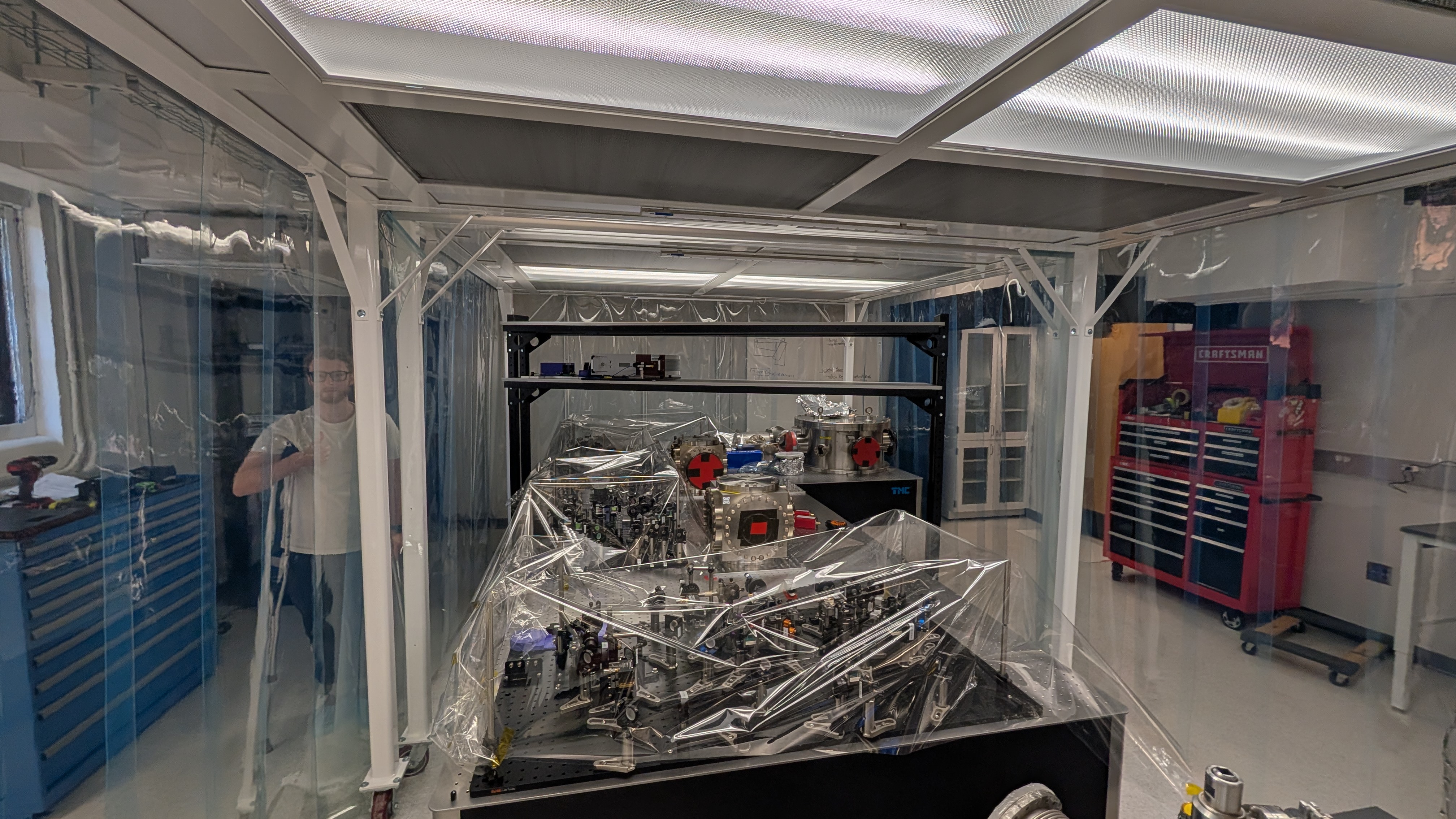
Following this tutorial: Laser Locking With Closed-Loop Transfer Function Measurement (liquidinstruments.com), here's a summary of useful points in measuring the transfer function of the plant, open loop system, etc, which can be useful in the design choices for the laser PID controller (like determining how good the gain parameters are). This was done with just the slow controller enabled. It would be a little more complicated if both slow and fast controllers are enabled because you would have to divide out the fast controller TF (from the Moku configuration, Out A of the LLB would not be the pure error signal). 

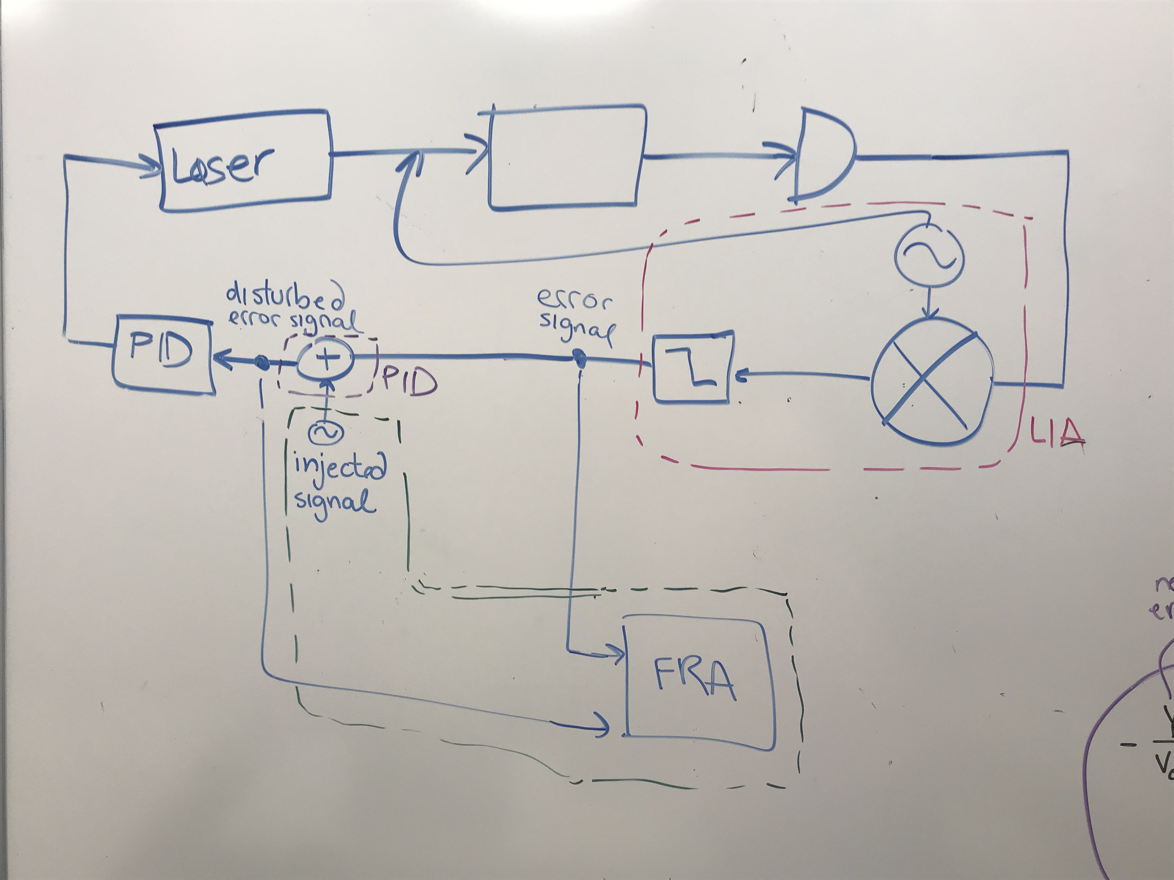
Note: there is an error in Figure 1 of the linked tutorial. Noise should be injected AFTER the plant for the subsequent math to be correct. 

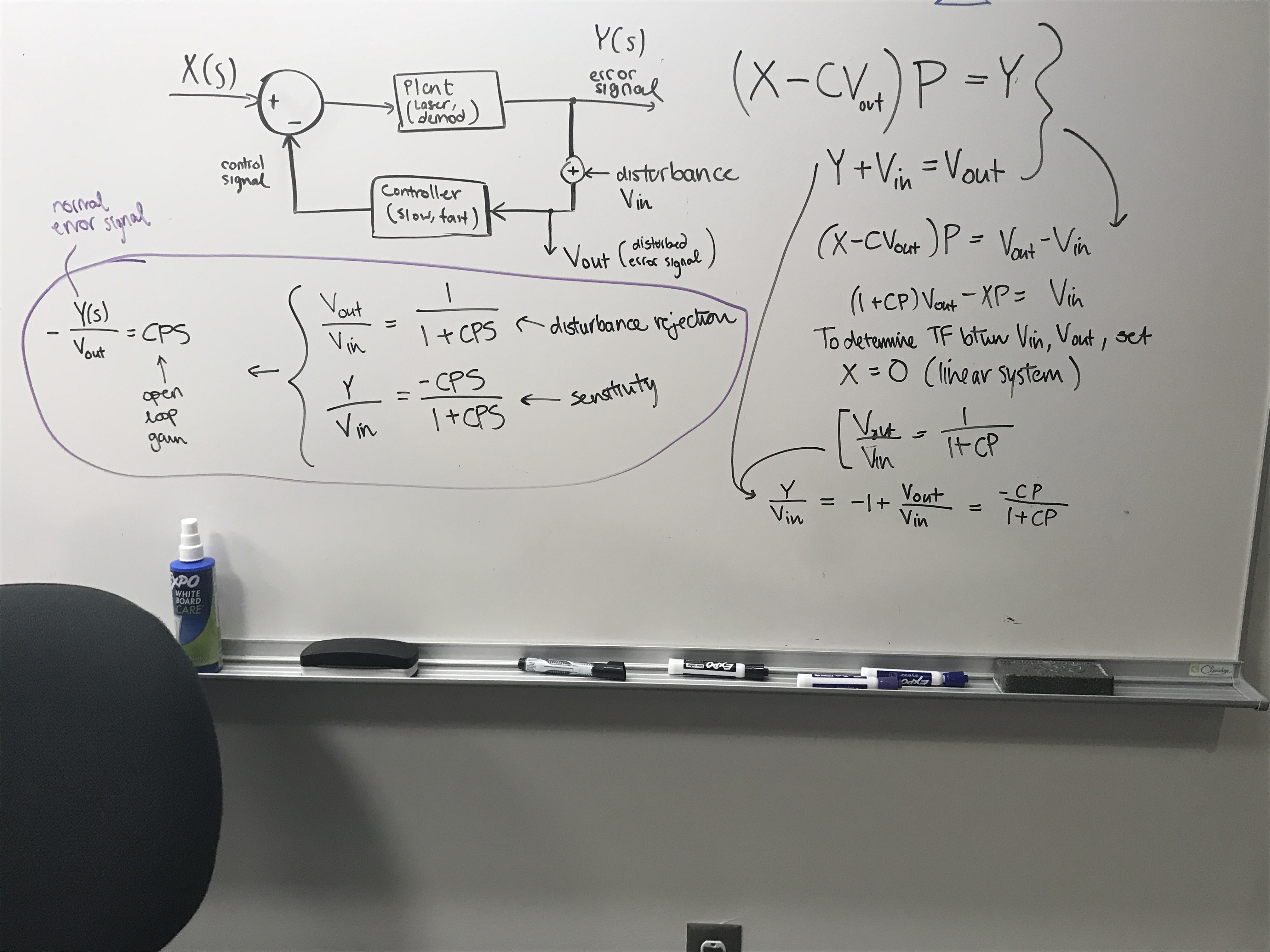
Basic idea: To test how good your plant can deal with disturbances, you inject some disturbance and measure the system response. A way to measure these responses is shown here: sys_tf.jpg (we combined the sensing S into the plant P, but the same math applies to the tutorial). Essentially, the math suggests that if we inject disturbances and measure their corresponding output, we can get the open and closed loop transfer function of the system, which informs us about the stability of our controller.

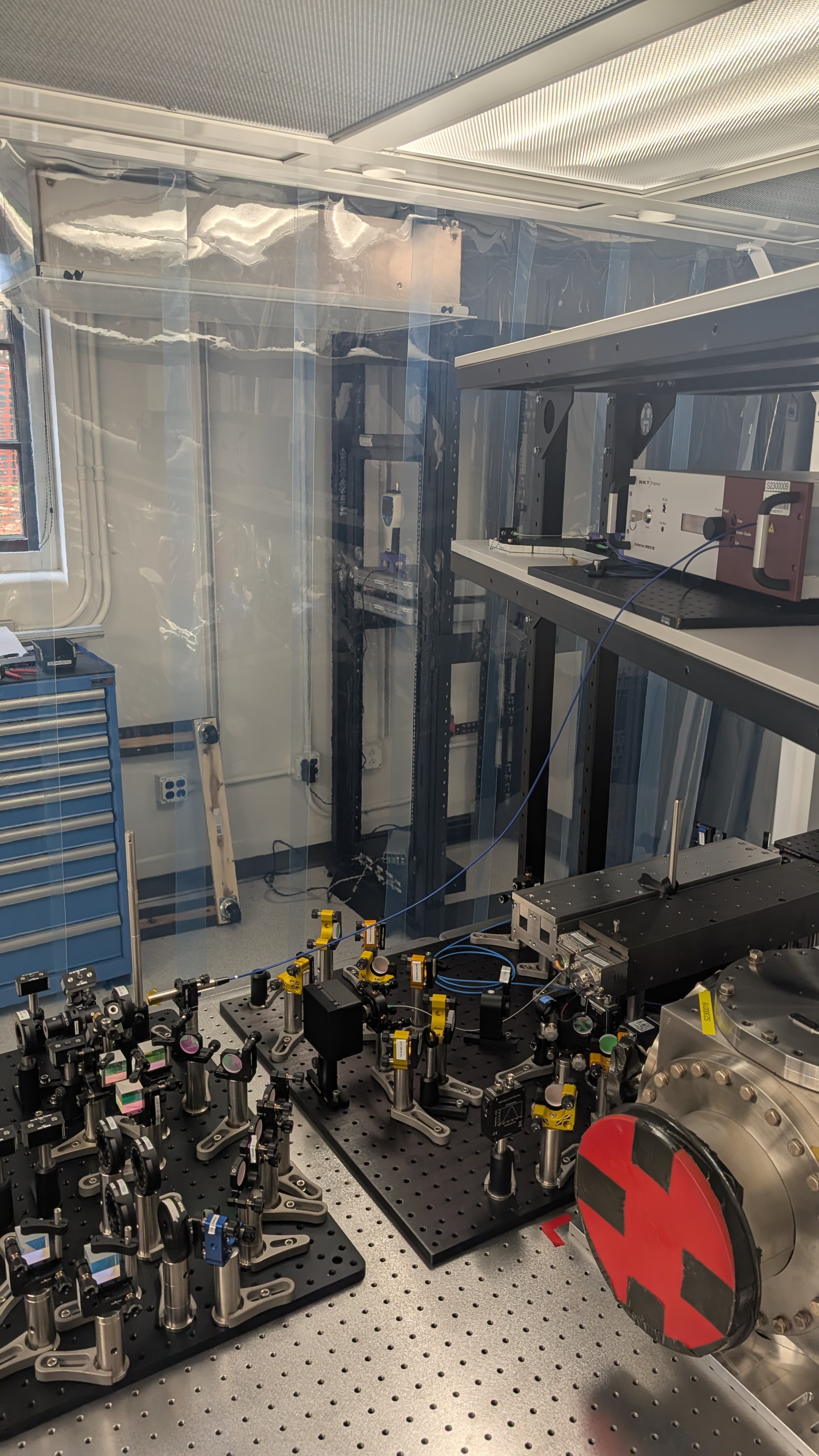
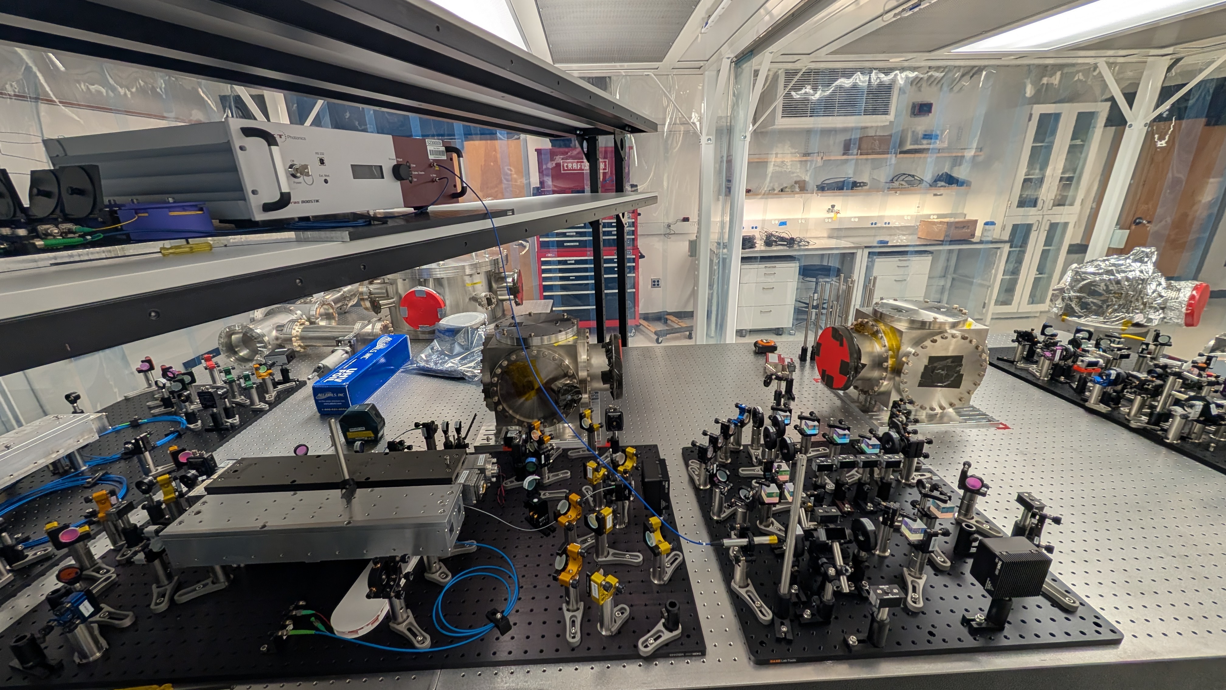
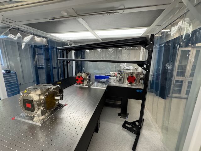
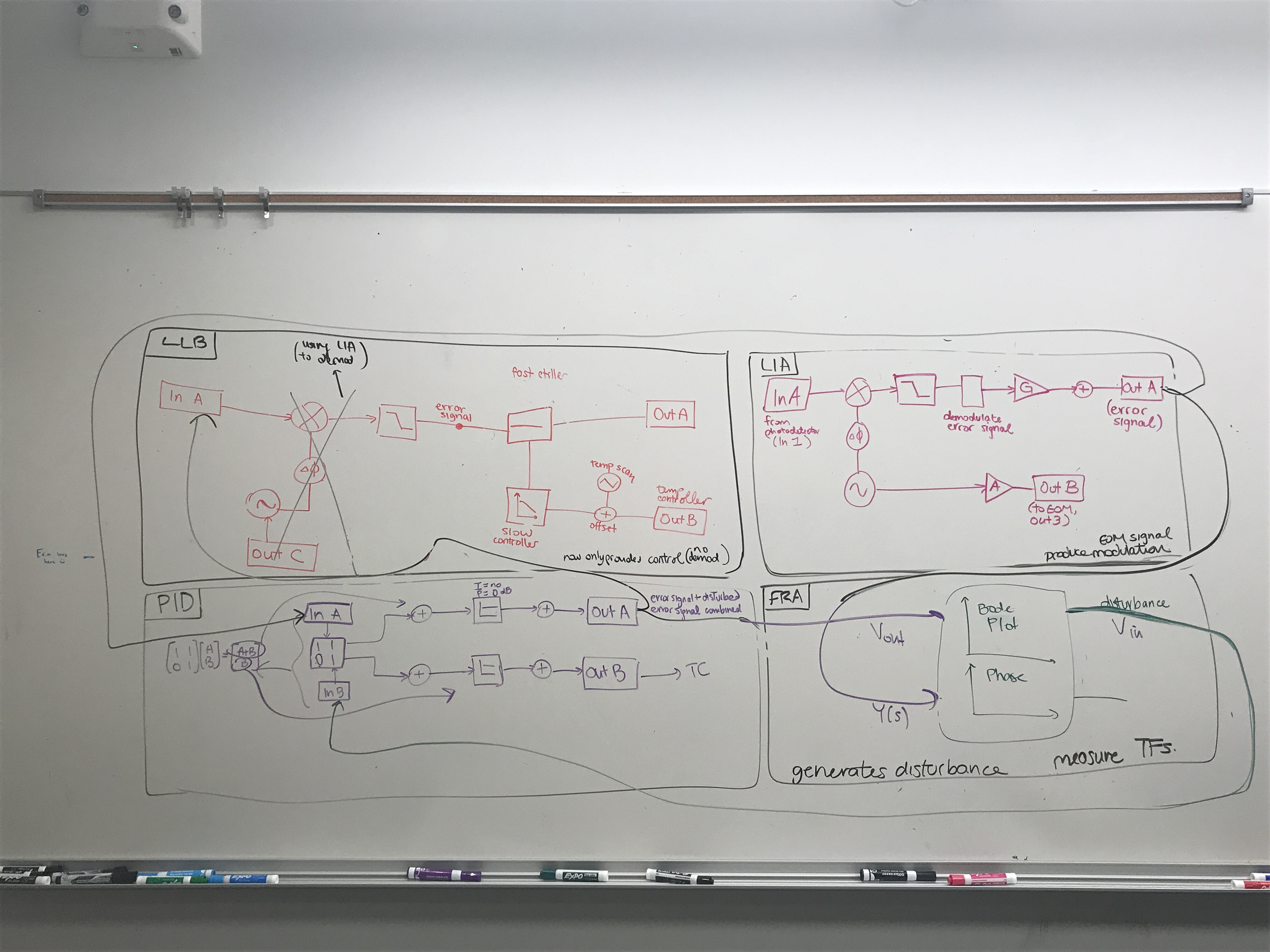
We need to split up the feedback loop into the following components to do this: schematic.jpg. We rigged up the Moku in this configuration to measure all these parameters: Mokuconfig.jpg, using the Laser Lock Box (LLB), Lock In Amplifier (LIA), PID, and Frequency Response Analyzer (FRA). You move the demodulation process into the Lock-In Amplifier (LIA) and perform the injection using a PID as an adder. Then, you use a Frequency Response Analyzer to get the bode plots for the different transfer functions (open loop, plant, etc). In the FRA, you apply a frequency scan to measure the transfer functions. 

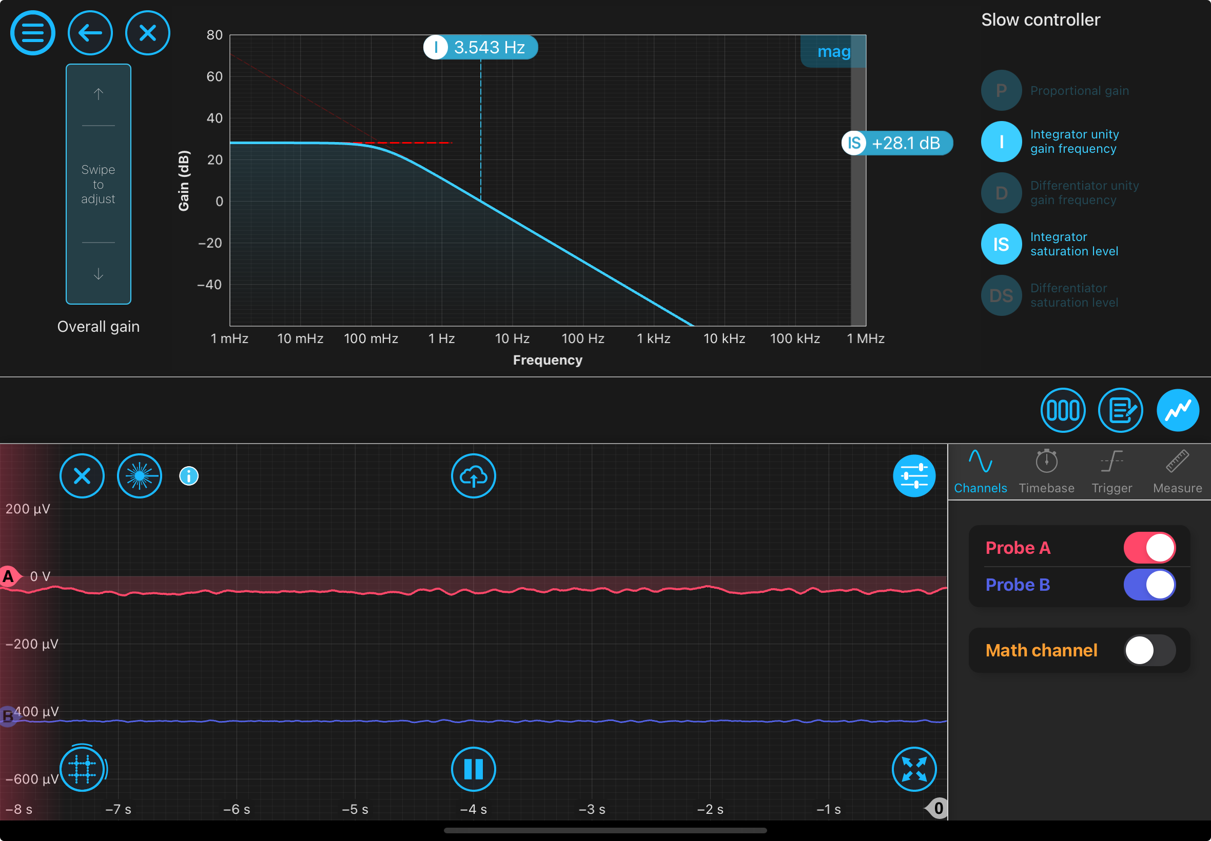
We locked the laser first using the following controller: slowcontroller.png. We measure the open loop transfer function (corrected for the phase going beyond 360 degrees), where we find unity gain (0 dB) occurs at 1.85 Hz with a phase margin of 65 deg: OpenLoopGainTransferFunction.pdf. This means that the system is reasonably stable (a large phase shift is needed to reach instability so the system is robust) and can control below 1.85Hz (can't suppress noise effectively above this).

This open loop TF is given by CP. We can divide CP by the controller transfer function (C) that we applied (dividing the gain and the phase) to get the plant transfer function, which is shown as a Bode plot here: PlantTransferFunction.pdf. A few notes:

• We divided OpenLoopGainTransferFunction.pdf by ControllerTF.pdf (controller bode plot) to get PlantTransferFunction.pdf (plant transfer function). Note that data for the open loop gain TF is not useful beyond ~12 Hz as seen in the noisy signal in the Bode plot (after unwrapping phase). So, we only consider the region of frequencies before 12 Hz in the plant transfer function bode plot.
• To divide the gain, you need to convert both transfer function Bode plots from the log scale of dB to amplitude (20 log (A) = dB) after which you can divide the two plots and reconvert back to dB (otherwise you divide by 0). 
• The plant transfer function is inclusive of the laser and entire demodulation process.
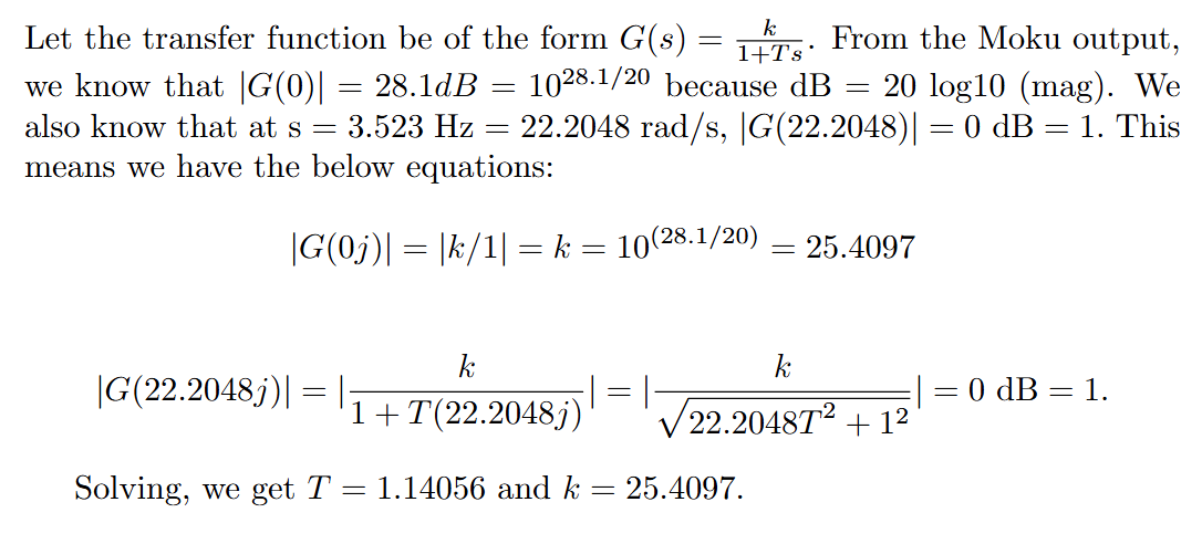
• Thanks Jeff for pointing out that we can figure out the controller based on these two parameters (unity gain frequency and initial magnitude) in the Moku output (slowcontroller.png). This is a first order controller as determined by the number of poles/zeros aka 1. Because there is one corner frequency from the Bode plot, we have G(s) = k / (1+Ts). The math is here (note: omega is in rad/s): math.png. So, our controller C(s) = G(s) = 25.4097/(1+1.14056s). I forgot to take a measure of the controller's phase plot so depending on the sign of -s or +s the controller phase plot is different. Anyways, this is the Bode plot of the controller we used to lock: ControllerTF.pdf. It matches the Moku controller Bode plot (slowcontroller.png). 
• Ian mentioned that the Moku's PID controller displayed is sometimes not reflective of the actual controller because the Moku has limits to its ability to implement the controller so we would use Jeff's code to correct the controller and get the right transfer function bode plot (I think). 

Knowing the plant TF, you can use these functions to find potential resonant peaks or bandwidth limits in the system. This is useful because you want to make sure your controller won't start to amplify those peaks and drive the system out of stable lock. The plant transfer function bode plot has a generally flat magnitude, which is expected because it should not be amplifying any particular frequency. The slight bump at ~4 Hz may be some slight resonance in the system, it shows up in the final noise spectrum as well interestingly enough (NoiseSpectra.pdf), although this is with the slow and fast controller. Ideally, you want the range of your open loop phase margin to be between -90 and 90 degrees for as large of a controller bandwidth as possible. We would be able to model the system fully if we could sum the noise spectra (inside closed loop) and plant transfer function. 

We can also check the goodness of our controller by looking at the disturbance rejection, which is the response put on a disturbance going through the system. You would want the bode plot of the disturbance rejection to be at low magnitude (e.g. negative dB) to suppress the disturbance. To ensure that the perturbations are suppressed enough and you can hold the lock with less noise, the magnitude of the disturbance rejection should not increase beyond 0 dB after the unity gain frequency because then, noise will be amplified in the system (i.e. (1/(1+CP))*N = disturbance rejection TF * Noise --> increased noise in the output). I don't really understand the last sentence of this article where the low frequency gain of the open loop TF matching the disturbance rejection magnitude suggests there is adequate noise suppression: I would think that as long as the magnitude of 1/(1+CP) is small, the magnitude of CP should not matter. 

I loaned a bag of Silver Plated 12 Point Bolts (1/4-28 x 7/8") with 1/4" washers, 25/pk to Paco. Duniway Part Number SBX-28-087. Paco said he would return the bag on Thursday, 9/26.