[Sander, Daniel, Torrey]
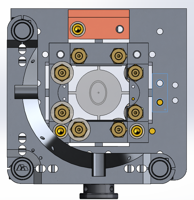
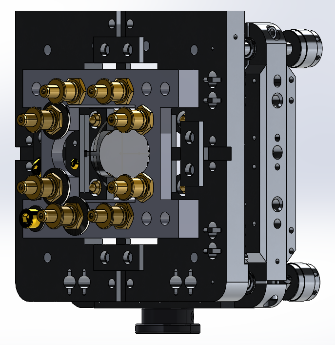
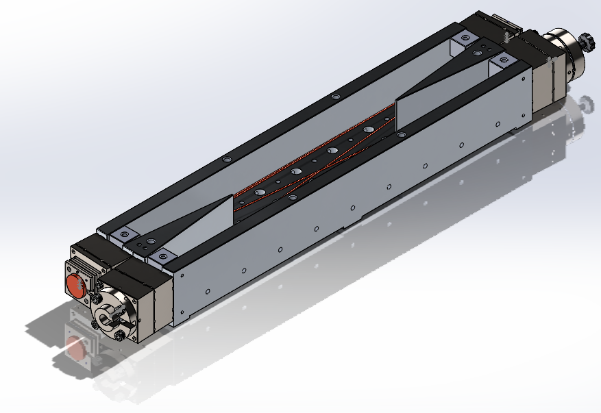
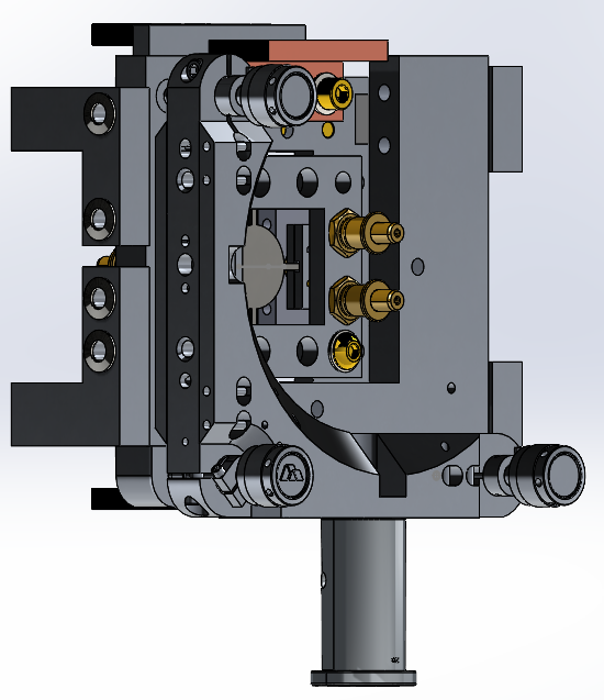
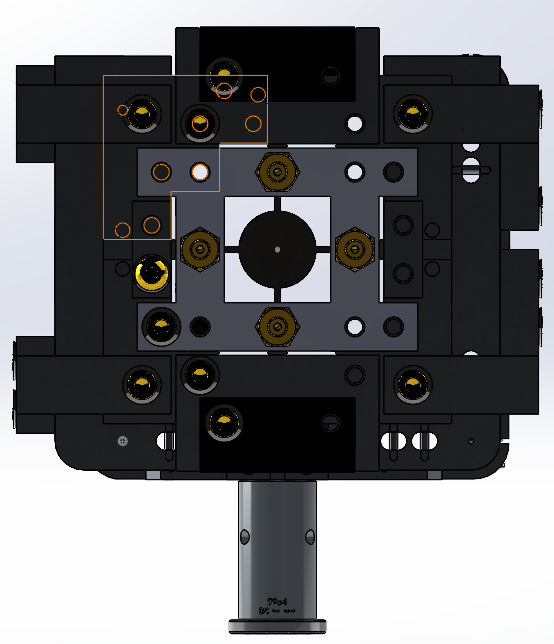
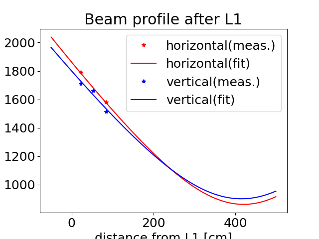
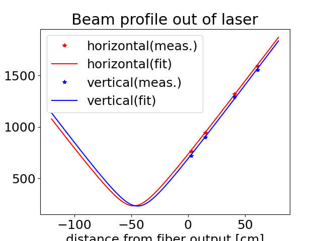
As discussed in group meeting, we tested the "mirror crusher" (the device that applies a force on a mirror in the filter cavities in order to change the radius of curvature of the optic, for wavefront control) yesterday. We first measured the beam profile and fit the data to the equation,
\[w^2(z) = w_0^2 + M^4 \left( (\frac{\lambda}{\pi w_0} \right)^2 (z-z_0)^2 \] ,
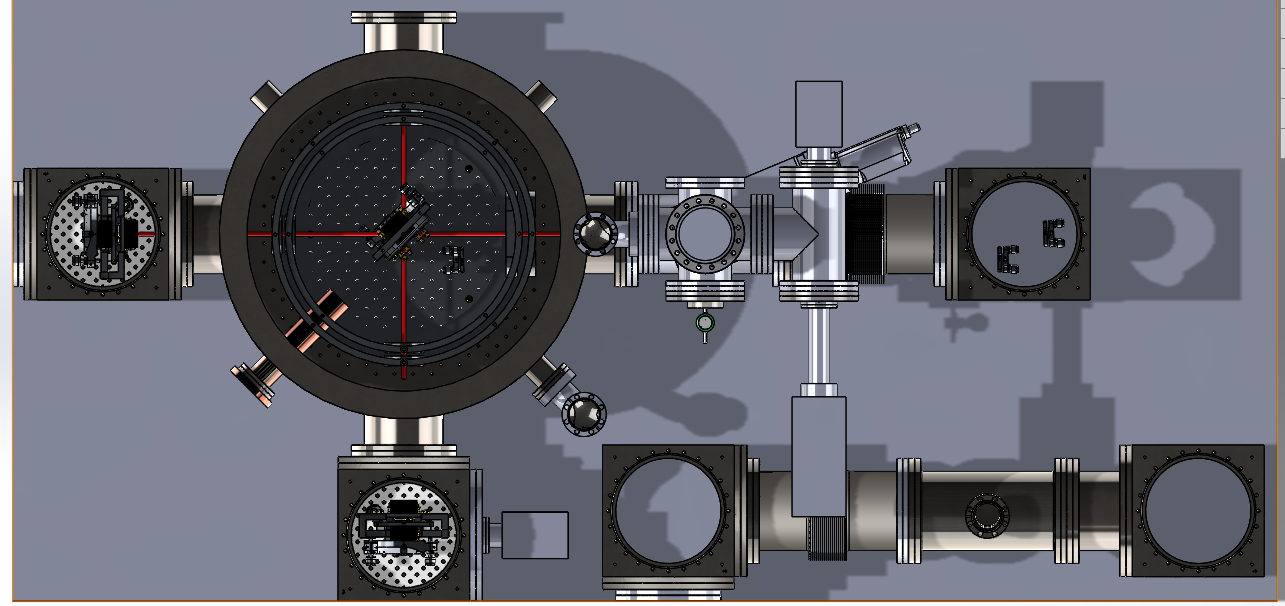
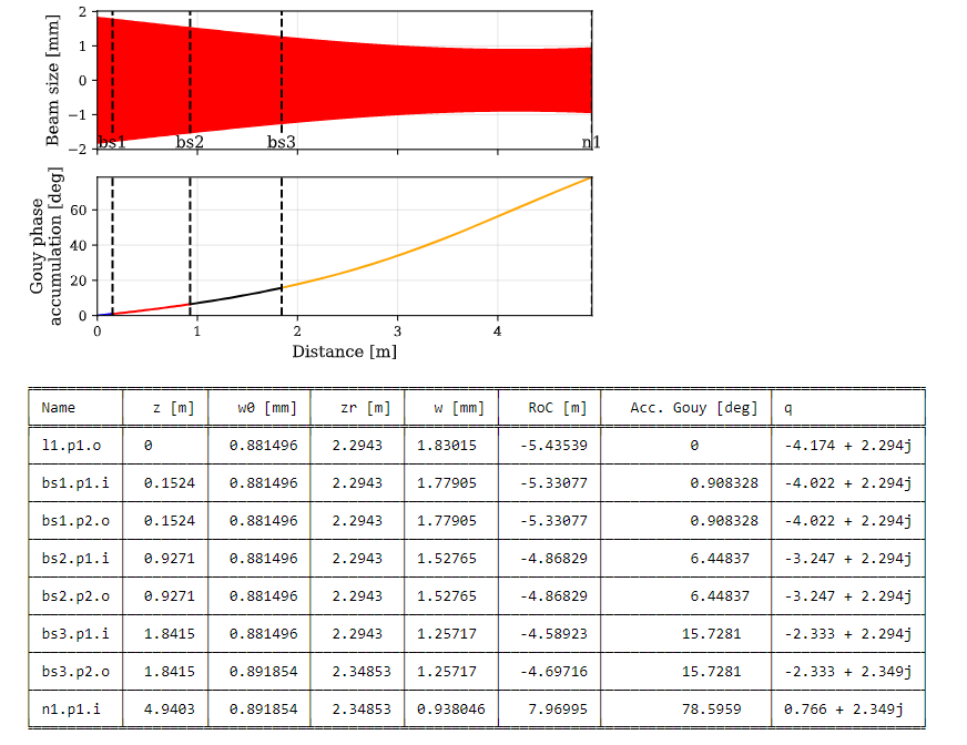
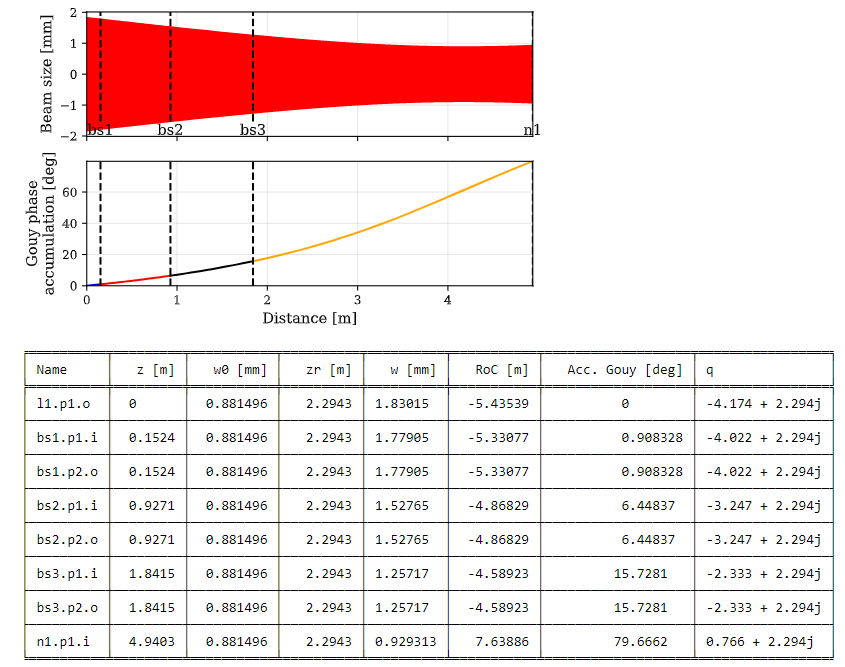
to get an approximate beam waist and location to use in the next step. The result for which can be found here.The optical layout of the system can be found here. We then wrote a quick code in Finesse to simulate the system, one for with a flat mirror, and then one for a curved mirror. The results for these can be found in the images attached labelled flat and curved respectfully. In the tables, the number of interest is under the w column, at the point n1.p1.i. This just corresponds to an arbitary point in space (where the scanning slit was placed). The difference of these values, and the estimated change in beam size from the crusher is then 38.1 microns. The actual measured change was (x,y): (17, 110). This discrepancy could come from the beam not being centered on the mirror being pushed on. Note that the model doesn't exactly agree with some of the experimental data in otherways, i.e. the expected beam diameter at the measurement point from the model is roughly 2 mm, where as the measured was ~2.7mm. I will update this post as the model is improved.
Additional improvements/iterations to be made:
-Maximize beamsize on optic thats being pushed on. Locate the waist some distance away. Then push on the mirror and see how the waist location changes.
-Improve collimation out of fiber. It is not collimated in the slightest, see here. We recently purchased a collimator that you can adjust along the z-axis to improve this. Will swap it out.

Adding the script used to model, version 1.